MIST

By Samuel Wharton (University of Leicester)

Magnetosheath jets are regions of enhanced solar wind density that form inside the magnetosheath and can locally compress the magnetopause, generating space weather effects. The higher density of the jet should result in it being brighter in soft X-rays due to the greater occurrence of the solar wind change exchange mechanism. It has been theorised by many authors they might be visible to a soft X-ray imager.
We simulated magnetosheath jets and calculated the X-ray flux expected from them at a soft X-ray imager. We found that it was difficult to resolve the jets due to the LOS integration effect and the noise within the images. However, viewing jets is more likely from viewing angles where the path length through the magnetosheath is short and there is a strong contrast between the jet and its surroundings in the image. Strong solar wind driving is also required so the emission is greater than the astrophysical background. This could be achieved with a larger telescope than SMILE-SXI that would be practical to build.

See publication for more details:
https://academic.oup.com/rasti/article/doi/10.1093/rasti/rzag059/8760917

Simulations of a magnetosheath jet seen from SMILE-SXI from three different viewing positions. The left column shows the intensity of X-rays entering the telescope. The middle column shows the expected count rate on the detector without noise. The right column shows a realistic image with Poisson noise applied.

By Mike Lockwood (University of Reading)

We have studied the evolution of the debris cloud generated by the high-altitude Anti-Satellite (ASAT) test on the Fengyun-1C satellite over the subsequent 18 years. More of the objects at sizes above 10cm have survived than was predicted four years after the ASAT test, despite the average space weather activity being higher than was assumed in making those predictions. We show how debris accelerated by the test into high-apogee orbits has acted as a reservoir, giving a long-lived supply of objects ready to start the reentry spiral. The average rate of descent varies with the solar cycle and with the solar rotation period because of the variation in EUV heating of the thermosphere. Geomagnetic storms
have a short-lived but significant effect on the altitude decay of the debris, the upper decile of geomagnetic activity accounting for 12% of the lost altitude at 400 km, rising to 19% at 700km. A second, more subtle, geomagnetic effect is seen to be present, identified as being driven by the Russell-McPherron effect on solar wind-magnetosphere couplingand thermospheric heating. The contribution of this mechanism to the semi-annual variation in average debris descent speed is greatest at high altitudes but other thermospheric effects, such as wave and tide dissipation and circulation changes, are more important at lower altitudes. At times of low solar activity the EUV heating is the dominant effect but the total geomagnetic contribution is more significant during disturbed times. We discuss how these results are of importance to controlled de-orbiting of space junk.

References
M. Lockwood, C. J. Scott, J. O'Donoghue, M. J. Owens, and L. A. Barnard (2026)
The contribution of the Russell-McPherron effect to the semiannual variation in thermospheric density, J. geophys. Res. Space Phys., 131, e2025JA034732, doi: 10.1029/2025JA034732
M. Lockwood (2025) The Celestial Rubbish Dump, Astronomy and Geophysics, 66 (3), 3.36–3.42, doi: 10.1093/astrogeo/ataf023

See publication for more details:
M. Lockwood, M.J. Owens, C. Saha, L.A. Barnard, C.J. Scott, and J. O’Donoghue (2026) Space Weather, Submitted

Comparison of days with predominant positive (left) and negative (right) IMF Y-component in the GSEQ frame. Parts A and D show the FY-1C debris descent speed, v, as a function of altitude, h, and fraction of a calendar year, F, where its annual variation due to Sun-Earth distance a (as a function of h) has been subtracted to reveal the semi-annual variation. Parts C and F show the height profiles of (v-a) at the dates of peak Russell-McPherron effect in March (green) and September (mauve). Parts B and E show the variation with F of the average (v-a) over the full height range. The Russell-McPherron effect enhances the March/September peak when the Y-component in GSEQ is negative/positive and so can be clearly seen to be driving a semi-annual variation in debris descent speed at higher altitudes.

By Neil Rogers (Lancaster University)

Many of us use the NASA “OMNI” database, which takes measurements from spacecraft (e.g., ACE or Wind) near the L1 Earth-Sun Lagrange point and uses them to predict solar wind conditions near the Earth’s bow shock nose. The question is: How accurate are these OMNI predictions? This is particularly topical given recent studies showing that measurement uncertainty could explain saturation in magnetospheric responses to solar wind driving (e.g., Sivadas et al. (2026), Nature, https://doi.org/10.1038/s41586-026-10757-4). We have compared 1-min resolution OMNI predictions of plasma density, velocity, and magnetic field with concurrent ‘ground truth’ measurements from two ESA Cluster spacecraft when they were located in the solar wind in years 2001 - 2023. After calibrating ‘systematic’ linear (instrumental) biases between pairs of spacecraft, we quantified and parameterised probability density functions (PDF) of the ‘stochastic’ differences between OMNI and Cluster. We found that many of these PDFs had a very narrow central peak (i.e., most differences were close to zero) but had ‘heavier tails’ in comparison with the Normal distribution (i.e., a greater likelihood of the largest differences). The Student’s-t distribution is a good fit for these cases, although we found the five-parameter Generalised Hyperbolic distribution provides the best characterisation of the rarest and largest differences (the outermost tails of the PDFs). Our paper provides a full quantification of both systematic and stochastic uncertainties, which could be used to place more realistic uncertainty bounds on analyses and forecasts that rely on OMNI data. Our database of times for which Cluster spacecraft were in the solar wind (~ 5000 hours) at various distances beyond the bow shock is also available to download: https://doi.org/10.5281/zenodo.18390327.

See publication for more details:
Rogers, N. C., Wild, J. A., & Grocott, A. (2026). Quantifying uncertainty in OMNI solar wind measurements projected from L1 to the Earth's bow shock. Journal of Geophysical Research: Space Physics, 131, e2026JA035221. https://doi.org/10.1029/2026JA035221

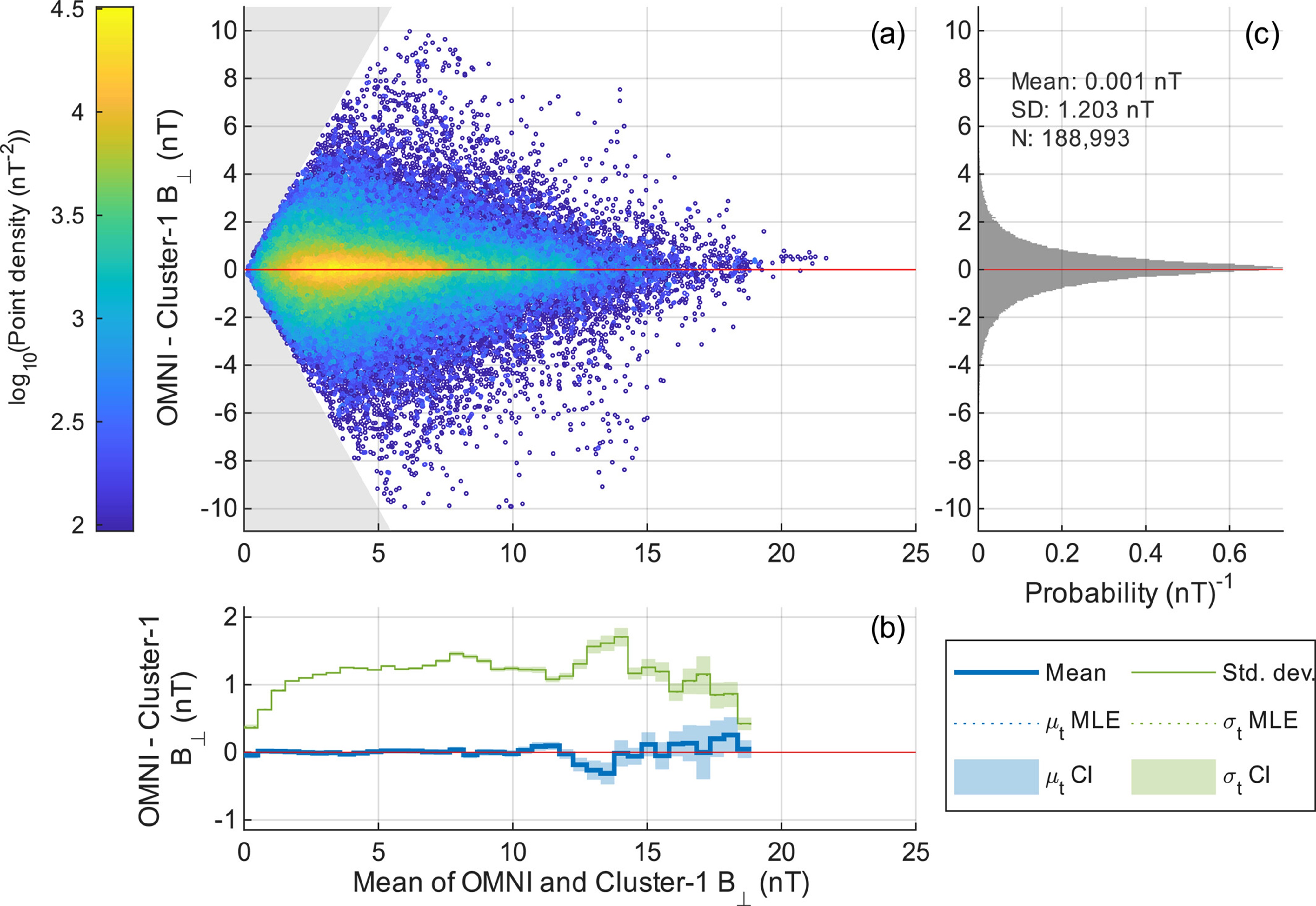
(a) Errors (OMNI minus Cluster-1) in the interplanetary magnetic field strength perpendicular to the Sun-Earth axis for all minutes in years 2001-2023. (b) Binned means and standard deviations of data in panel (a) and coefficients of fitted truncated Normal distributions (maximum likelihood estimates and 95% confidence intervals). (c) PDF of data in panel (a).

How Can Turbulence Improve Space Weather Forecasts?

By Cara Waters (Queen Mary University of London)

The auroral electrojet (AE) index is one of the key indicators of high latitude geomagnetic activity. Forecasting it from upstream solar wind conditions remains challenging due to nonlinear coupling and multiscale variability. To combat this, we test whether incorporating solar wind turbulence improves short timescale AE forecasts beyond models based on solely the mean solar wind and interplanetary magnetic field. We compare two gradient boosted decision tree (XGBoost) models using near-Earth solar wind observations from OMNI. The baseline model uses standard mean field, density and velocity parameters, while the turbulence-aware model adds measures of fluctuation amplitude, intermittency, energy partition, compressibility, and Alfvénic structure. Both models achieve a peak performance at short lead times, giving correlations above 0.8 at 60 minutes. However, the turbulence-aware model maintains forecasting skill for longer lead times. The turbulence-aware model also provides consistent improvements over both the baseline model and persistence. Critically, this model improves forecast robustness for high-impact events. Using cost-loss analysis, the baseline model provides decreasing economic value with increasing AE threshold. In contrast, the turbulence-aware model maintains an approximately constant threshold for positive economic value, indicating stable economic usefulness even for extreme AE conditions. Using interpretable machine learning techniques, we can show that the most important turbulence parameters for this at short timescales are fluctuations in Bz and the skew of these fluctuations, and at longer timescales it is the properties of the turbulence (cross helicity, compressibility, and residual energy). This demonstrates that turbulence provides complementary, scale-dependent information beyond mean solar wind parameters, improving both forecast performance and decision-relevant value for operational space weather applications.

See publication for more details:

Cara L. Waters, Christopher H. K. Chen, Mathew J. Owens (2026). Beyond Mean Solar Wind Conditions: Turbulence-Aware Forecasting of the AE Index. Space Weather, 24(7). https://doi.org/10.1029/2026SW005094

Potential economic value 𝑉 against cost/loss ratio 𝑟 for the base model in (a) and turbulence model in (b), for a range of thresholds of auroral electrojet (AE) between 800 and 1,200 nT. (c) The 𝑥-intercept of each of the curves plotted against the threshold AE index for the turbulence model (red circles) and the base model (blue squares).