MIST
Magnetosphere, Ionosphere and Solar-Terrestrial
Latest articles
- Temporal Variability of Saturn's H2 Dayglow and Northern Aurora Observed by Hisaki and Cassini
- The Jupiter Auroral Ionosphere Code
- Analysis of Chorus Wave Power on Burst‐Mode Timescales During the Van Allen Probes Era
- Soft X-Ray Emission from Saturn's Magnetosheath II: Solar Wind Driving
- Which Kelvin-Helmholtz waves grow along the spatially-varying magnetopause flanks and why?
Latest news
Open Letter Ready For Signatories
Protect MIST Science! Sign the MIST Community Open Letter on the STFC funding cuts!
https://sites.google.com/view/uk-mist-community-open-letter
Statement from MIST Council regarding the STFC Funding Situation
Statement from MIST Council regarding the STFC Funding Situation
MIST Council is deeply concerned by the ongoing STFC funding uncertainty and its impact on our community and beyond.
The current combination of prospective delayed and reduced funding, together with already volatile financial situations at universities across the UK, is placing significant strain on research groups. In some cases, institutions may be unable to support researchers through gaps between projects, increasing precarity across the community and adding significant pressure on early-career researchers.
We are concerned that continued uncertainty risks accelerating a brain drain from the UK, as skilled researchers reconsider their future in a system offering limited stability. The loss of expertise at any career stage would have lasting consequences for UK space science.
What is going on?
For those that are unaware of the situation, it is complex and evolving. We suggest the following sources to get up to speed on the current developments.
https://ras.ac.uk/news-and-press/news/proposed-budget-cuts-catastrophe-uk-astronomy
What are we doing about it?
Behind the scenes, MIST Council is actively engaging with relevant parties to understand the scale of the challenge and to identify constructive ways forward.
- We are seeking seasoned members of the community to join MIST Council on a task force to help develop options and represent the needs of our community. If you would like to be involved, please reach out to us via the MIST Council email (This email address is being protected from spambots. You need JavaScript enabled to view it.) by the end of this week (13th February 2026).
- In addition to the task force, we want to provide an open forum for discussion and collective input among all members of the wider MIST community. We are exploring options and will be in touch as soon as possible with further details.
- We believe in working together in the face of the current challenges and we are collaborating with UKSP and others to strive for a fair and positive outcome for all. We are reaching out to members of the SSAP (Solar System Advisory Panel) to explore the hosting of a community town hall meeting, like the one already being organised by the AAP (Astronomy Advisory Panel), to provide an open forum for discussion and collective input.
What can you do to help?
There are several open letters representing people in various career stages that have been made available to sign. We encourage you to read the relevant letter(s) and to sign them if you support them:
- Fellowship Holders: https://advancedfellows-openletter-stfc.github.io/index.html
- Early Career Researchers: https://ecr-openletter-stfc.github.io/
The Royal Astronomical Society are also urging Fellows to lobby their MPs against the cuts, and have included a template letter that can be used to do so:
https://ras.ac.uk/news-and-press/news/ras-fellows-urged-lobby-against-unprecedented-cuts
MIST Council will continue to advocate for transparency, stability, and funding structures that recognise both the long-term nature of our science and the people who deliver it.
We thank you for your continued support in this period of uncertainty.
Please contact This email address is being protected from spambots. You need JavaScript enabled to view it. if you have further suggestions.
MIST Council
![]()
Announcement of New MIST Council 2025
We are very pleased to announce the following members of the community have been elected to MIST Council:
- Gemma Bower (University of Leicester), MIST Councillor
- Tom Elsden (University of St Andrews), MIST Councillor
- Cameron Patterson (Lancaster University), MIST Councillor
- Fiona Ball (University of Southampton), Student Representative
They will begin their terms in July 2025.
We thank outgoing MIST Council members: Maria Walach, Chiara Lazzeri and Emma Woodfield. Andy Smith will remain on council a little longer as a co-opted member to cover Rosie Johnson's maternity leave.
The current composition of Council can be found on our website (https://www.mist.ac.uk/community/mist-council).
Announcement of New MIST Councillors.
We are very pleased to announce the following members of the community have been elected unopposed to MIST Council:
- Rosie Johnson (Aberystwyth University), MIST Councillor
- Matthew Brown (University of Birmingham), MIST Councillor
- Chiara Lazzeri (MSSL, UCL), Student Representative
Rosie, Matthew, and Chiara will begin their terms in July. This will coincide with Jasmine Kaur Sandhu, Beatriz Sanchez-Cano, and Sophie Maguire outgoing as Councillors.
The current composition of Council can be found on our website, and this will be amended in July to reflect this announcement (https://www.mist.ac.uk/community/mist-council).
Nominations are open for MIST Council
We are very pleased to open nominations for MIST Council. There are three positions available (detailed below), and elected candidates would join Georgios Nicolaou, Andy Smith, Maria-Theresia Walach, and Emma Woodfield on Council. The nomination deadline is Friday 31 May.
Council positions open for nomination
2 x MIST Councillor - a three year term (2024 - 2027). Everyone is eligible.
MIST Student Representative - a one year term (2024 - 2025). Only PhD students are eligible. See below for further details.
About being on MIST Council
If you would like to find out more about being on Council and what it can involve, please feel free to email any of us (email contacts below) with any of your informal enquiries! You can also find out more about MIST activities at mist.ac.uk. Two of our outgoing councillors, Beatriz and Sophie, have summarised their experiences being on MIST Council below.
Beatriz Sanchez-Cano (MIST Councillor):
"Being part of the MIST council for the last 3 years has been a great experience personally and professionally, in which I had the opportunity to know better our community and gain a larger perspective of the matters that are important for the MIST science progress in the UK. During this time, I’ve participated in a number of activities and discussions, such as organising the monthly MIST seminars, Autumn MIST meetings, writing A&G articles, and more importantly, being there to support and advise our colleagues in cases of need together with the wonderful council members. MIST is a vibrant and growing community, and the council is a faithful reflection of it."
Sophie Maguire (MIST Student Representative):
"Being the student representative for MIST council has been an amazing experience. I have been part of organizing conferences, chairing sessions, and writing grant applications based on the feedback MIST has received. From a wider perspective, MIST has helped to grow and support my professional networks which in turn, directly benefits my PhD work as well. I would encourage any PhD student to apply for the role of MIST Student Representative and I would be happy to answer any questions or queries you have about the role."
How to nominate
If you would like to stand for election or you are nominating someone else (with their agreement!) please email This email address is being protected from spambots. You need JavaScript enabled to view it. by Friday 31 May. If there is a surplus of nominations for a role, then an online vote will be carried out with the community. Please include the following details in the nomination:
- Name
- Position (Councillor/Student Rep.)
- Nomination Statement (150 words max including a bit about the nominee and focusing on your reasons for nominating. This will be circulated to the community in the event of a vote.)
MIST Council details
- Sophie Maguire, University of Birmingham, Earth's ionosphere - This email address is being protected from spambots. You need JavaScript enabled to view it.
- Georgios Nicolaou, MSSL, solar wind plasma - This email address is being protected from spambots. You need JavaScript enabled to view it.
- Beatriz Sanchez-Cano, University of Leicester, Mars plasma - This email address is being protected from spambots. You need JavaScript enabled to view it.
- Jasmine Kaur Sandhu, University of Leicester, Earth’s inner magnetosphere - This email address is being protected from spambots. You need JavaScript enabled to view it.
- Andy Smith, Northumbria University, Space Weather - This email address is being protected from spambots. You need JavaScript enabled to view it.
- Maria-Theresia Walach, Lancaster University, Earth’s ionosphere - This email address is being protected from spambots. You need JavaScript enabled to view it.
- Emma Woodfield, British Antarctic Survey, radiation belts - This email address is being protected from spambots. You need JavaScript enabled to view it.
- MIST Council email - This email address is being protected from spambots. You need JavaScript enabled to view it.
Nuggets of MIST science, summarising recent papers from the UK MIST community in a bitesize format.
If you would like to submit a nugget, please fill in the following form: https://forms.gle/Pn3mL73kHLn4VEZ66 and we will arrange a slot for you in the schedule. Nuggets should be 100–300 words long and include a figure/animation. Please get in touch!
If you have any issues with the form, please contact This email address is being protected from spambots. You need JavaScript enabled to view it..
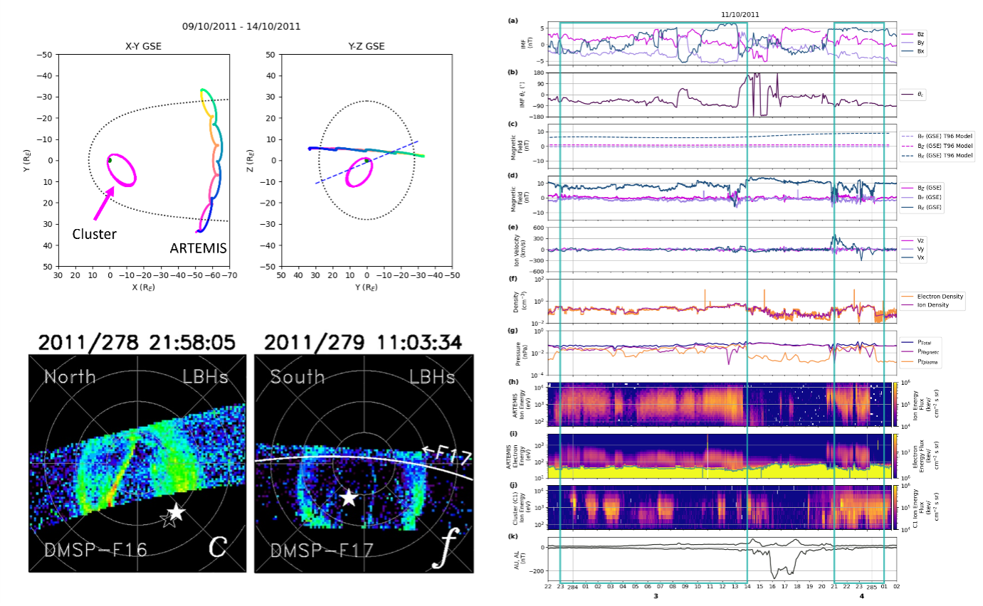
Plasma observations in the high-latitude and distant magnetotail associated with cusp-aligned arcs during intervals of northward IMF
By Michaela Mooney and Steve Milan (University of Leicester)
During periods of northward interplanetary magnetic field (IMF), the magnetospheric structure and dynamics are dramatically different and less understood compared to the southward IMF case.
Under northward IMF magnetic reconnection occurs at higher latitudes tailward of the cusp, known as lobe reconnection (Dungey, 1963). Lobe reconnection can occur on the same IMF field line in both hemispheres, known as dual lobe reconnection. It is thought that dual lobe reconnection can result in either the partial or complete closure of the magnetosphere (Milan et al., 2022). The auroral oval is also contracted to higher latitudes reflecting the reduced open flux content of the magnetosphere. The auroral emission is dimmer and distinct auroral features are observed poleward of the auroral oval such as cusp-aligned arcs, horse collar aurora and transpolar arcs.
Using Cluster and ARTEMIS in-situ data, we examined a period of prolonged northward IMF during which multiple instances of cusp-aligned arcs were observed poleward of the auroral oval. The Cluster observations showed trapped plasma on closed flux in the high latitude magnetotail (|ZGSE| ~ 13 RE) in regions which would typically be expected to be open magnetotail lobe void of plasma under southward IMF. Meanwhile, the ARTEMIS spacecraft observed simultaneous high electron and ion fluxes in the distant magnetotail (XGSE ~ - 60 RE). The plasma in both magnetotail regions was observed coincidently with observations of cusp-aligned arcs in the auroral data. We interpret these observations of trapped plasma on closed field lines as providing the source population for the cusp-aligned arc emission in the polar region.
During this interval we suggest that the magnetosphere was almost entirely closed as a result of dual lobe reconnection. The magnetotail is closed or partially closed but extends at least as far as ∼ 60 RE downtail. The occurrence of plasma in the magnetotail and the closure of the magnetosphere resulted in distinct changes to the magnetotail structure including a reduction in the magnetic field strength and pressure as well as a narrowing of the tail by approximately 20 RE.
See the full papers for further details:
Milan, S. E., Mooney, M. K., Bower, G. E., Taylor, M. G. G. T., Paxton, L. J., Dandouras, I., et al. (2023). The association of cusp-aligned arcs with plasma in the magnetotail implies a closed magnetosphere. Journal of Geophysical Research: Space Physics, 128, e2023JA031419. https://doi. org/10.1029/2023JA031419
Mooney, M. K., Milan, S. E., & Bower, G.E. (2024). Plasma observations in the distant magnetotail during intervals of northward IMF. Journal of Geophysical Research: Space Physics, 129,e2023JA031999. https://doi.org/10.1029/2023JA031999
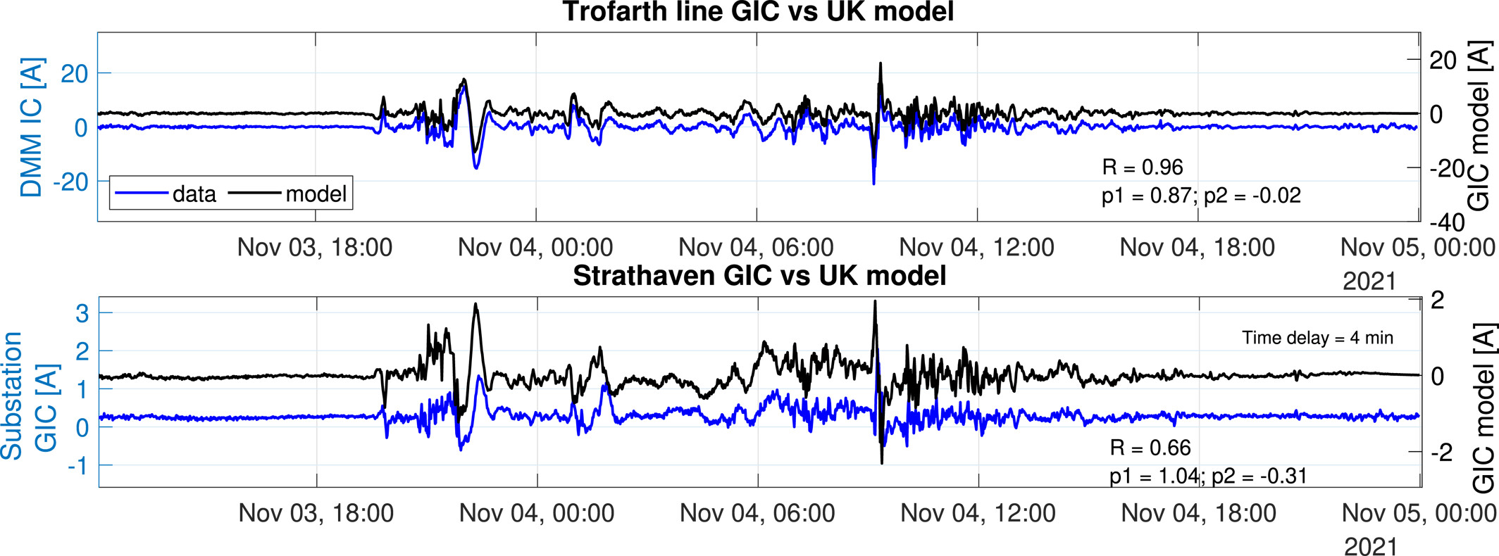
Validating GIC models in the UK using Differential Magnetometer and Magnetotelluric Data
By Juliane Huebert (British Geological Survey)
Geomagnetically induced currents (GICs) are a well-known consequence of increased geomagnetic activity due to solar storms. They pose the risk of damaging ground-based infrastructure like the high voltage power transmission network, gas pipelines and railways. Large-scale models of GICs in the UK exist, taking into account geomagnetic data, the induced ground electric fields and the configuration of the ground-based technologies. Validating these complex models is not easy and requires independent observations. To measure GICs in the HV voltage power network, we applied the Differential Magnetometer Method (DMM) at several sites in Britain. At each site, one magnetometer was placed under the power lines while a second one was located a few hundred meters away. By looking at the difference in the data between the two we can isolate the direct current flowing in the power lines. Data were recorded for several months, catching periods of increased geomagnetic activity. We then compared the measured current strength to the BGS GIC model developed from open source data sets of the UK power grid. The model also uses a measure for the ground electrical conductivity that is based on so-called magnetotelluric (MT) measurements which we performed in a country-wide campaign. MT data is necessary to characterize the spatial changes in the ground electric field due to local geology. We found our model and the field measurements to match very well, giving confidence that our simulations of the whole UK grid are very close to the correct values.
See full paper for further details:
Hübert, J., Beggan, C. D., Richardson, G. S., Gomez-Perez, N., Collins, A., & Thomson, A. W. P. (2024). Validating a UK geomagnetically induced current model using differential magnetometer measurements. Space Weather, 22, e2023SW003769. https://doi.org/10.1029/2023SW003769
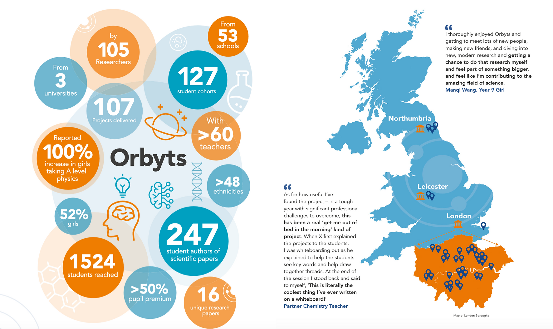
Orbyts Impact Report
By Jasmine Sandhu (University of Leicester)
Orbyts is a multi-award winning movement that partners scientists with schools to empower school students to undertake world-leading research. In this MIST nugget, we are delighted to present Orbyts very first Impact Report!
Read the Orbyts Impact Report 2017-2023 here: https://www.orbyts.org/impact
Over the past six years we have seen the programme enable a transformational impact on young people, researchers and teachers alike and we’re excited to share that with you here.
To date, Orbyts has created 100+ research partnerships, empowering 1500+ school students. We’ve increased inclusivity in post-16 STEM uptake, where students Orbyts engaged are 50+% girls, 50+% pupil premium, and identified from 48+ ethnicities. We have grown with new Hubs in North East England and Leicester, alongside expansion of our London Hub.
Read the report for all the statistics on Orbyts, spotlights on the ground-breaking research being led by students, and all the exciting plans for Orbyts in 2024!
We’d like to extend our thanks to all those who have and continue to support Orbyts, without whom this work would not be possible. In particular we would like to thank all the researchers and teachers for all their time and hard work. We also gratefully acknowledge support from all of our funders, including the UCL Access and Widening Participation Office, the Ogden Trust, UK Space Agency, European Research Council, EPSRC, and STFC.
Orbyts currently sits precariously positioned with no financial support beyond our upcoming 2024 programme. If you think that Orbyts might be something you would like to support, then we would love to hear from you at This email address is being protected from spambots. You need JavaScript enabled to view it..
Read the Orbyts Impact Report 2017-2023 for further details: https://www.orbyts.org/impact.
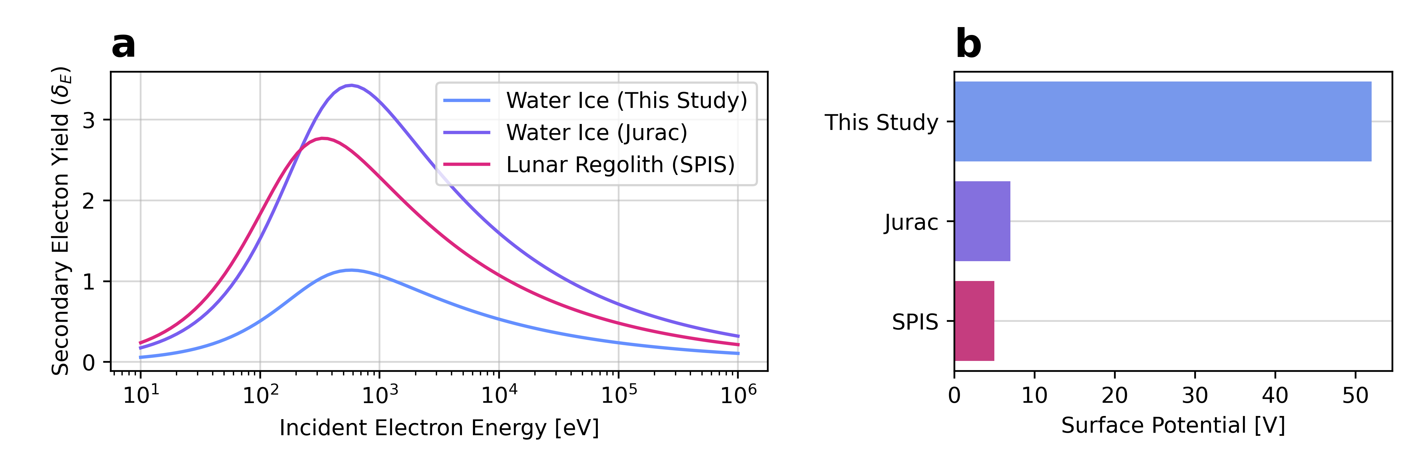
Surface Charging of Jupiter's Moon Europa
By Sachin Reddy (UCL / National Institute of Polar Research)
Jupiter’s moon Europa is exposed to a constant flow of plasma from its own ionosphere and the Jovian magnetosphere, which consists of a thermal and suprathermal population. As these particles flow onto the surface, an electrostatic potential forms in accordance with Kirchhoff’s current law. In this study, we investigate the electric charging of Europa’s icy surface using 3D particle-in-cell simulations via the Spacecraft Plasma Interactions Software (SPIS).
We find that surface potentials on Europa vary from -14 to -52 V. They change as a function of Europa’s four hemispheres, the solar illumination conditions, the plasma environment, and the properties of the surface itself. We reveal that the presence of an ionospheric plasma population reduces the surface potentials, producing a “dampening effect”. We also find that secondary electron emission is a crucial mechanism in Europan charging, shifting potentials by an order of magnitude for the same plasma properties. We argue that additional laboratory work into Europa-like-ice electron emission is necessary to reduce the uncertainties in the modelling. These results could be both corroborated and improved upon by the upcoming Europa Clipper and JUICE missions, and may be of use in the design of future missions to Europa’s surface (e.g. landers or other robotic explorers).
See full paper for further details:
Reddy, Sachin A., Nordheim, Tom N. and Harris, Camilla, D.K.,. "Surface Charging of Jupiter’s Moon Europa." The Astrophysical Journal Letters 962.2 (2024): L29. https://doi.org/10.3847/2041-8213/ad251e
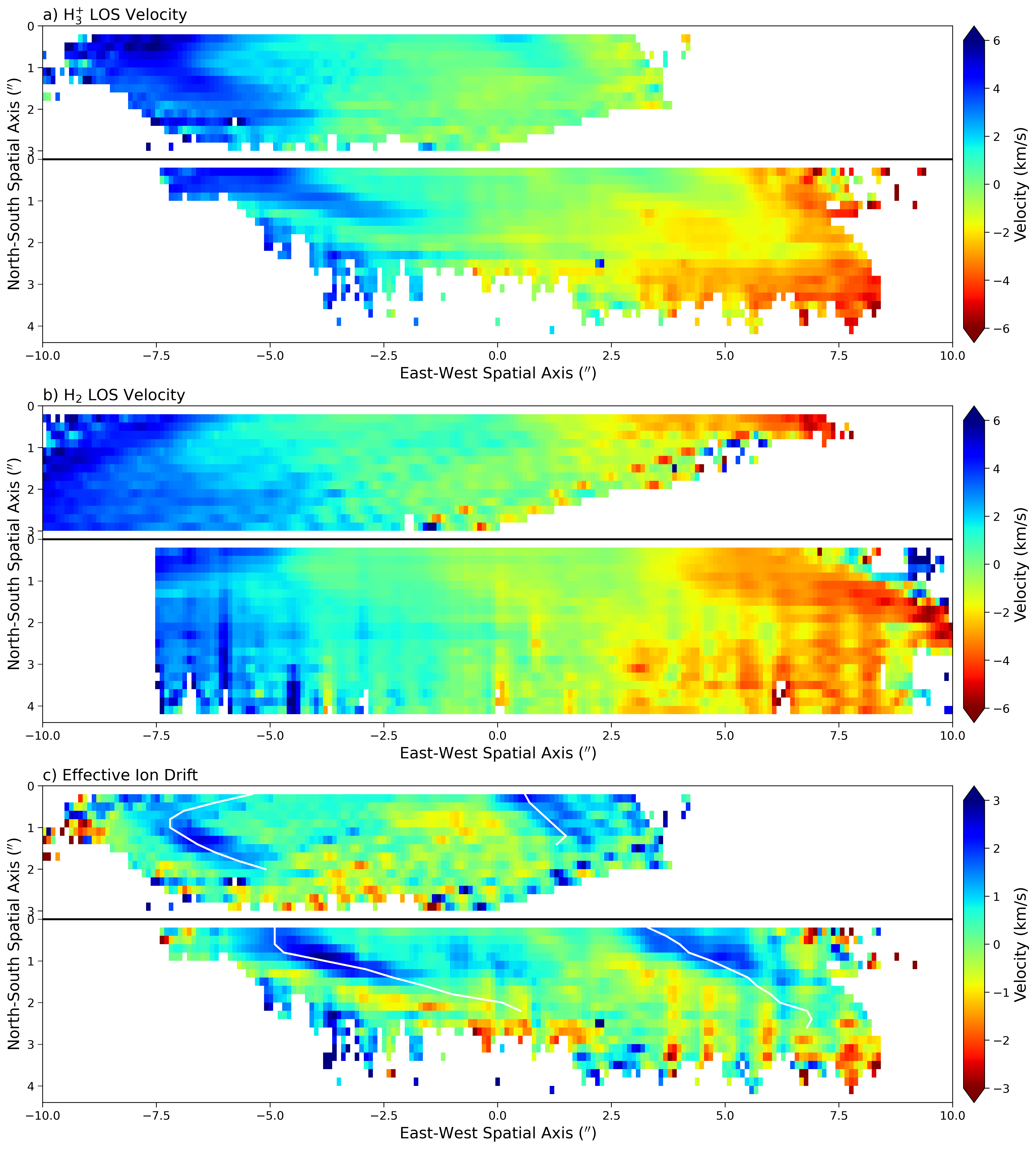
Asymmetric Ionospheric Jets in Jupiter's Aurora
By Ruoyan Wang (University of Leicester)
We have simultaneously observed line-of-sight ionospheric and thermospheric winds in Jupiter using the Keck II telescope and produced one of the first global maps of both ion and neutral flows in the same layer of any atmosphere. Since ionospheric currents are through the relative motion of ions within the neutral atmosphere, comparing these two maps produces a global map of the "effective" ion drifts, the E x B flows that drive upper ionospheric currents. To the surprise of the Jupiter community, this upper atmospheric "effective" ion drift is dominated by two sunward blue-shifted jets associated with the dawn and dusk main auroral region, highly reminiscent of ionospheric flows seen on Earth. This discovery is directly opposite to the expected rotationally symmetric breakdown in corotation driven by the plasma-heavy magnetosphere. Our result suggests that the asymmetric currents close in the upper ionosphere, while the closure of breakdown-in-corotation currents occurs deep in the lower ionosphere, resulting in powerful upward auroral currents penetrating through overlying regions of downward currents associated with the asymmetric currents. Such a mechanism could potentially explain the complex switching generation of Jupiter's main auroral emissions observed by the Juno mission. Moreover, this study highlights the importance of the neutral atmosphere and interactions between ions and neutrals on other planets, including Earth, making Jupiter an important global comparator for future studies of these interactions.
See full paper for further details:
Wang, R., Stallard, T. S., Melin, H., Baines, K. H., Achilleos, N., Rymer, A. M., Ray, R. C., Nichols, J. D., Moore, L., O'Donoghue, J., Chowdhury, M. N., Thomas, E. M., Knowles, K. L., Tiranti, P. I., Miller, S. (2023). Asymmetric Ionospheric Jets in Jupiter's Aurora. Journal of Geophysical Research: Space Physics, 128, e2023JA031861. https://doi.org/10.1029/2023JA031861.