MIST
Magnetosphere, Ionosphere and Solar-Terrestrial
Latest articles
- Temporal Variability of Saturn's H2 Dayglow and Northern Aurora Observed by Hisaki and Cassini
- The Jupiter Auroral Ionosphere Code
- Analysis of Chorus Wave Power on Burst‐Mode Timescales During the Van Allen Probes Era
- Soft X-Ray Emission from Saturn's Magnetosheath II: Solar Wind Driving
- Which Kelvin-Helmholtz waves grow along the spatially-varying magnetopause flanks and why?
Latest news
Open Letter Ready For Signatories
Protect MIST Science! Sign the MIST Community Open Letter on the STFC funding cuts!
https://sites.google.com/view/uk-mist-community-open-letter
Statement from MIST Council regarding the STFC Funding Situation
Statement from MIST Council regarding the STFC Funding Situation
MIST Council is deeply concerned by the ongoing STFC funding uncertainty and its impact on our community and beyond.
The current combination of prospective delayed and reduced funding, together with already volatile financial situations at universities across the UK, is placing significant strain on research groups. In some cases, institutions may be unable to support researchers through gaps between projects, increasing precarity across the community and adding significant pressure on early-career researchers.
We are concerned that continued uncertainty risks accelerating a brain drain from the UK, as skilled researchers reconsider their future in a system offering limited stability. The loss of expertise at any career stage would have lasting consequences for UK space science.
What is going on?
For those that are unaware of the situation, it is complex and evolving. We suggest the following sources to get up to speed on the current developments.
https://ras.ac.uk/news-and-press/news/proposed-budget-cuts-catastrophe-uk-astronomy
What are we doing about it?
Behind the scenes, MIST Council is actively engaging with relevant parties to understand the scale of the challenge and to identify constructive ways forward.
- We are seeking seasoned members of the community to join MIST Council on a task force to help develop options and represent the needs of our community. If you would like to be involved, please reach out to us via the MIST Council email (This email address is being protected from spambots. You need JavaScript enabled to view it.) by the end of this week (13th February 2026).
- In addition to the task force, we want to provide an open forum for discussion and collective input among all members of the wider MIST community. We are exploring options and will be in touch as soon as possible with further details.
- We believe in working together in the face of the current challenges and we are collaborating with UKSP and others to strive for a fair and positive outcome for all. We are reaching out to members of the SSAP (Solar System Advisory Panel) to explore the hosting of a community town hall meeting, like the one already being organised by the AAP (Astronomy Advisory Panel), to provide an open forum for discussion and collective input.
What can you do to help?
There are several open letters representing people in various career stages that have been made available to sign. We encourage you to read the relevant letter(s) and to sign them if you support them:
- Fellowship Holders: https://advancedfellows-openletter-stfc.github.io/index.html
- Early Career Researchers: https://ecr-openletter-stfc.github.io/
The Royal Astronomical Society are also urging Fellows to lobby their MPs against the cuts, and have included a template letter that can be used to do so:
https://ras.ac.uk/news-and-press/news/ras-fellows-urged-lobby-against-unprecedented-cuts
MIST Council will continue to advocate for transparency, stability, and funding structures that recognise both the long-term nature of our science and the people who deliver it.
We thank you for your continued support in this period of uncertainty.
Please contact This email address is being protected from spambots. You need JavaScript enabled to view it. if you have further suggestions.
MIST Council
![]()
Announcement of New MIST Council 2025
We are very pleased to announce the following members of the community have been elected to MIST Council:
- Gemma Bower (University of Leicester), MIST Councillor
- Tom Elsden (University of St Andrews), MIST Councillor
- Cameron Patterson (Lancaster University), MIST Councillor
- Fiona Ball (University of Southampton), Student Representative
They will begin their terms in July 2025.
We thank outgoing MIST Council members: Maria Walach, Chiara Lazzeri and Emma Woodfield. Andy Smith will remain on council a little longer as a co-opted member to cover Rosie Johnson's maternity leave.
The current composition of Council can be found on our website (https://www.mist.ac.uk/community/mist-council).
Announcement of New MIST Councillors.
We are very pleased to announce the following members of the community have been elected unopposed to MIST Council:
- Rosie Johnson (Aberystwyth University), MIST Councillor
- Matthew Brown (University of Birmingham), MIST Councillor
- Chiara Lazzeri (MSSL, UCL), Student Representative
Rosie, Matthew, and Chiara will begin their terms in July. This will coincide with Jasmine Kaur Sandhu, Beatriz Sanchez-Cano, and Sophie Maguire outgoing as Councillors.
The current composition of Council can be found on our website, and this will be amended in July to reflect this announcement (https://www.mist.ac.uk/community/mist-council).
Nominations are open for MIST Council
We are very pleased to open nominations for MIST Council. There are three positions available (detailed below), and elected candidates would join Georgios Nicolaou, Andy Smith, Maria-Theresia Walach, and Emma Woodfield on Council. The nomination deadline is Friday 31 May.
Council positions open for nomination
2 x MIST Councillor - a three year term (2024 - 2027). Everyone is eligible.
MIST Student Representative - a one year term (2024 - 2025). Only PhD students are eligible. See below for further details.
About being on MIST Council
If you would like to find out more about being on Council and what it can involve, please feel free to email any of us (email contacts below) with any of your informal enquiries! You can also find out more about MIST activities at mist.ac.uk. Two of our outgoing councillors, Beatriz and Sophie, have summarised their experiences being on MIST Council below.
Beatriz Sanchez-Cano (MIST Councillor):
"Being part of the MIST council for the last 3 years has been a great experience personally and professionally, in which I had the opportunity to know better our community and gain a larger perspective of the matters that are important for the MIST science progress in the UK. During this time, I’ve participated in a number of activities and discussions, such as organising the monthly MIST seminars, Autumn MIST meetings, writing A&G articles, and more importantly, being there to support and advise our colleagues in cases of need together with the wonderful council members. MIST is a vibrant and growing community, and the council is a faithful reflection of it."
Sophie Maguire (MIST Student Representative):
"Being the student representative for MIST council has been an amazing experience. I have been part of organizing conferences, chairing sessions, and writing grant applications based on the feedback MIST has received. From a wider perspective, MIST has helped to grow and support my professional networks which in turn, directly benefits my PhD work as well. I would encourage any PhD student to apply for the role of MIST Student Representative and I would be happy to answer any questions or queries you have about the role."
How to nominate
If you would like to stand for election or you are nominating someone else (with their agreement!) please email This email address is being protected from spambots. You need JavaScript enabled to view it. by Friday 31 May. If there is a surplus of nominations for a role, then an online vote will be carried out with the community. Please include the following details in the nomination:
- Name
- Position (Councillor/Student Rep.)
- Nomination Statement (150 words max including a bit about the nominee and focusing on your reasons for nominating. This will be circulated to the community in the event of a vote.)
MIST Council details
- Sophie Maguire, University of Birmingham, Earth's ionosphere - This email address is being protected from spambots. You need JavaScript enabled to view it.
- Georgios Nicolaou, MSSL, solar wind plasma - This email address is being protected from spambots. You need JavaScript enabled to view it.
- Beatriz Sanchez-Cano, University of Leicester, Mars plasma - This email address is being protected from spambots. You need JavaScript enabled to view it.
- Jasmine Kaur Sandhu, University of Leicester, Earth’s inner magnetosphere - This email address is being protected from spambots. You need JavaScript enabled to view it.
- Andy Smith, Northumbria University, Space Weather - This email address is being protected from spambots. You need JavaScript enabled to view it.
- Maria-Theresia Walach, Lancaster University, Earth’s ionosphere - This email address is being protected from spambots. You need JavaScript enabled to view it.
- Emma Woodfield, British Antarctic Survey, radiation belts - This email address is being protected from spambots. You need JavaScript enabled to view it.
- MIST Council email - This email address is being protected from spambots. You need JavaScript enabled to view it.
Nuggets of MIST science, summarising recent papers from the UK MIST community in a bitesize format.
If you would like to submit a nugget, please fill in the following form: https://forms.gle/Pn3mL73kHLn4VEZ66 and we will arrange a slot for you in the schedule. Nuggets should be 100–300 words long and include a figure/animation. Please get in touch!
If you have any issues with the form, please contact This email address is being protected from spambots. You need JavaScript enabled to view it..
Modeling and Observations of the Effects of the Alfvén Velocity Profile on the Ionospheric Alfvén Resonator
By Rosie Hodnett (University of Leicester)
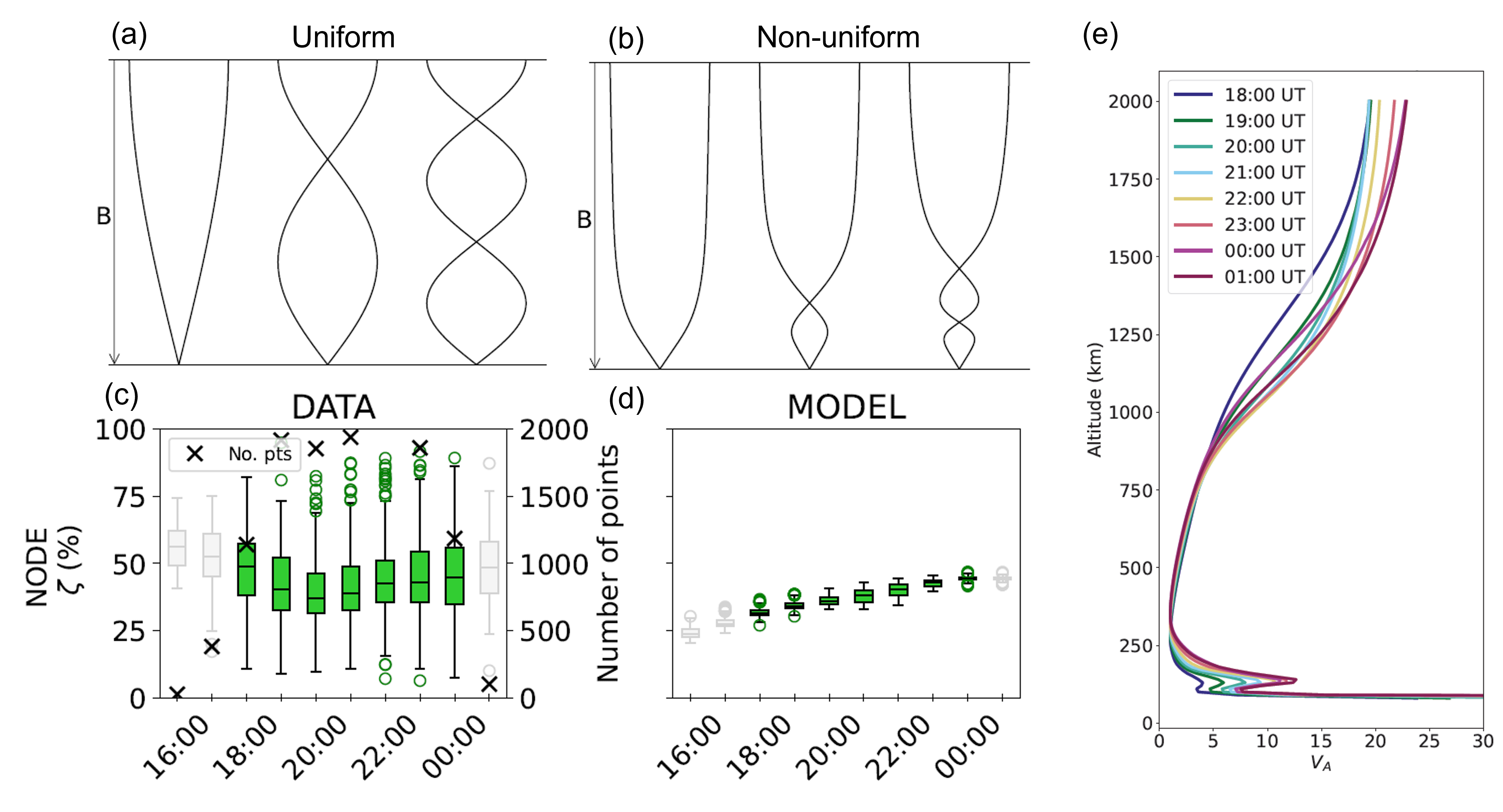
The Ionospheric Alfvén Resonator (IAR) occurs when Alfvén waves partially reflect from boundaries in the ionosphere, towards the bottom of the ionosphere and above the F-region peak. The frequencies of the IAR are strongly controlled by the plasma mass density in the ionosphere, which is not uniform.
We have observed IAR in induction coil magnetometer data at Eskdalemuir, UK (BGS site), and extracted the harmonic frequencies for nine years of data. To model the harmonic frequencies, we used the International Reference Ionosphere and the International Geomagnetic Reference Field to model Alfvén velocity profiles. By solving a one-dimensional wave equation, we modelled the first five harmonics of the IAR for times where we had data. The wave structure of the electric field for a uniform case is shown in panel (a), and the resulting modelled harmonics for a non-uniform case is shown in panel (b). We modelled the frequencies with the lower boundary condition of the electric field of the wave being a node (shown in the figure below) and an antinode. By looking at the percentage difference between the fundamental frequency and the average separation of the harmonics (ζ) for both the node and antinode models and comparing this with the data, we find that the lower boundary is closest to being a node. ζ is presented for the node case, with UT, in panels (c) and (d), which show the data and the model respectively, binned by UT. The trend of increasing ζ towards midnight is due to changing Alfvén velocity profiles (shown in panel (e)), and suggests that the ionosphere is becoming more non-uniform. As such, measurements of IAR could be used to gain insight into the shape of the Alfvén velocity profile of the ionosphere.
BGS induction coil magnetometer data, search for 'induction coil': https://webapps.bgs.ac.uk/services/ngdc/
accessions/index.html
See publication for further information:
Hodnett, R. M., Yeoman, T. K., Beggan, C. D., & Wright, D. M. (2024). Modeling and observations of the effects of the Alfvén velocity profile on the Ionospheric Alfvén Resonator. Journal of Geophysical Research: Space Physics, 129, e2023JA032308. https://doi.org/10.1029/2023JA032308
Topology of turbulence within collisionless plasma reconnection
Bogdan Hnat (University of Warwick)
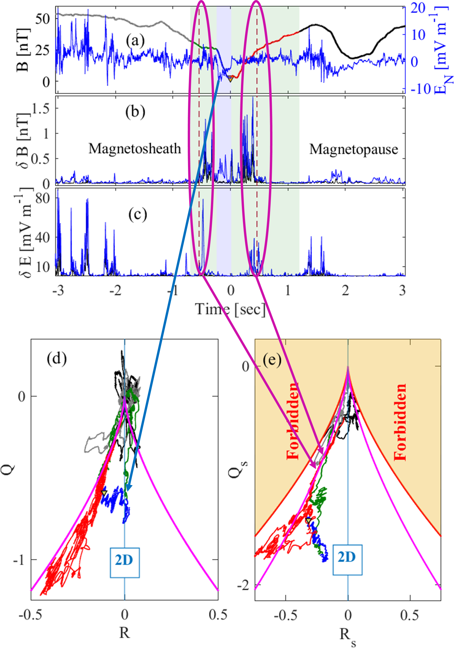
Collisionless magnetic reconnection [1] and plasma turbulence [2] are fundamental mechanisms that transfer energy across scales and between electromagnetic fields and particles. Stretched turbulent vortices and thin reconnection current sheets are prime sites of plasma heating and particle acceleration. Magnetic field line topology is central to both these processes.
We have classified the magnetic field topology observed as the four MMS spacecraft fly through a well resolved reconnection site. The MMS spacecraft separation defines a spatial 'yardstick', which is of order of the ion inertial range di, for sampling magnetic field topology. However, spatial variation of the topology is indirectly captured on a much finer spatial scale due to high time resolution of the magnetic field measurements, 8192 samples per second.
We find two distinct types of the magnetic field line topology near and at the electron dissipation region (EDR). At the edges of the EDR turbulent-like topology, identical to the topology of stretched vortices in hydrodynamic turbulence, is dominant. It coincides with large high-frequency electromagnetic perturbations. At the EDR the topology departs from turbulence and the structures appear to be two-dimensional, coinciding with suppression of electromagnetic fluctuations. The topology of the magnetic field line directly orders electron acceleration and heating. Suprathermal electrons are absent where turbulent-like topology dominates, but the bulk electron temperature anisotropy is enhanced. Reduced two-dimensional topology at the EDR coincides with the suprathermal electrons. The turbulent-like topology can arise in EMHD in scales smaller than electron inertial scale when vorticity dominates the dynamics. We find that vorticity is indeed dominant at all times within our interval.
References:
[1] J. Birn, E.R. Priest, Reconnection of Magnetic Fields: Magnetohydrodynamics and Collisionless Theory and Observations (Cambridge University Press, New York, 2007).
[2] Matthaeus, W.H. and Velli, M.,Space Science Reviews, 160(1), pp.145-168 (2011).
See publication for further information:
Hnat, Bogdan, Sandra Chapman, and Nicholas Watkins. "Topology of turbulence within collisionless plasma reconnection." Scientific Reports 13.1 (2023): 18665.
Plasma vorticity in the high-latitude ionosphere
By Gareth Chisham (British Antarctic Survey)
Measurements of ionospheric plasma flow vorticity can be used for studying ionospheric plasma transport processes, such as convection and turbulence, over a wide range of spatial scales. This study presents an analysis of probability density functions (PDFs) of ionospheric vorticity for selected regions of the northern hemisphere high-latitude ionosphere as measured by the Super Dual Auroral Radar Network (SuperDARN) over a 6-year interval (2000-2005 inclusive). Making certain assumptions, the observed asymmetric vorticity PDFs can be decomposed into two separate components: (1) A single-sided function that results from the large-scale vorticity inherent in the ionospheric convection pattern, driven by magnetic reconnection; (2) A symmetric double-sided function that results from meso-scale vorticity that derives from fluid processes such as turbulence, and from measurement uncertainties.
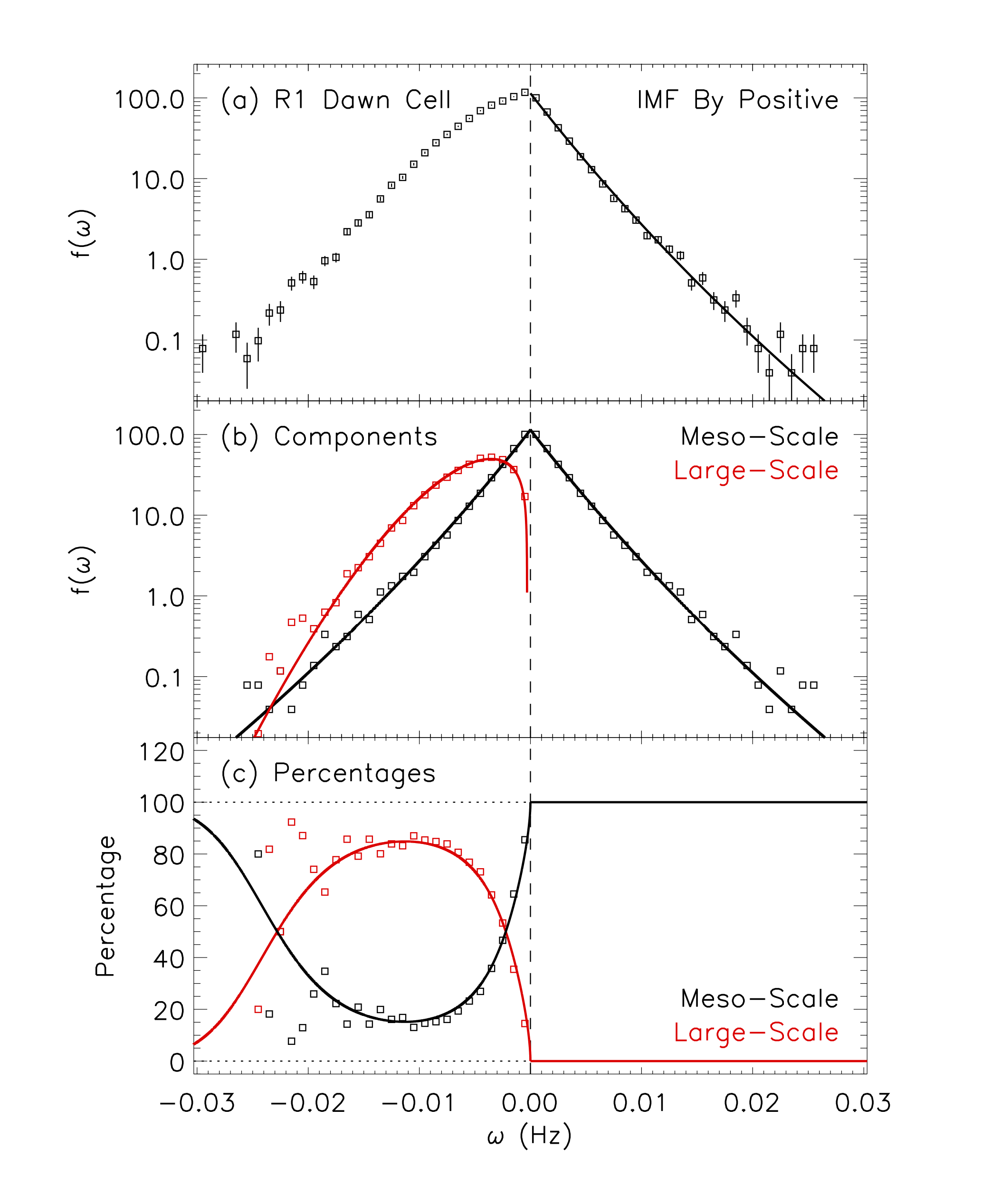
Being able to model ionospheric vorticity in this way will help to improve models of ionospheric plasma flow that are often used in larger-scale system models. At the present time, these plasma flow models typically only consider the larger-scale convection flow. Our observation of a significant meso-scale flow vorticity component due to turbulence will have implications for the fidelity of these models.
See paper for further details: Chisham, G. and Freeman, M. P. (2023). Separating contributions to plasma vorticity in the high-latitude ionosphere from large-scale convection and meso-scale turbulence. Journal of Geophysical Research: Space Physics, 128, e2023JA031885, https://doi.org/10.1029/2023JA031885.
Detection of the northern infrared aurora at Uranus using the W.M. Keck II Telescope and NIRSPEC instrument
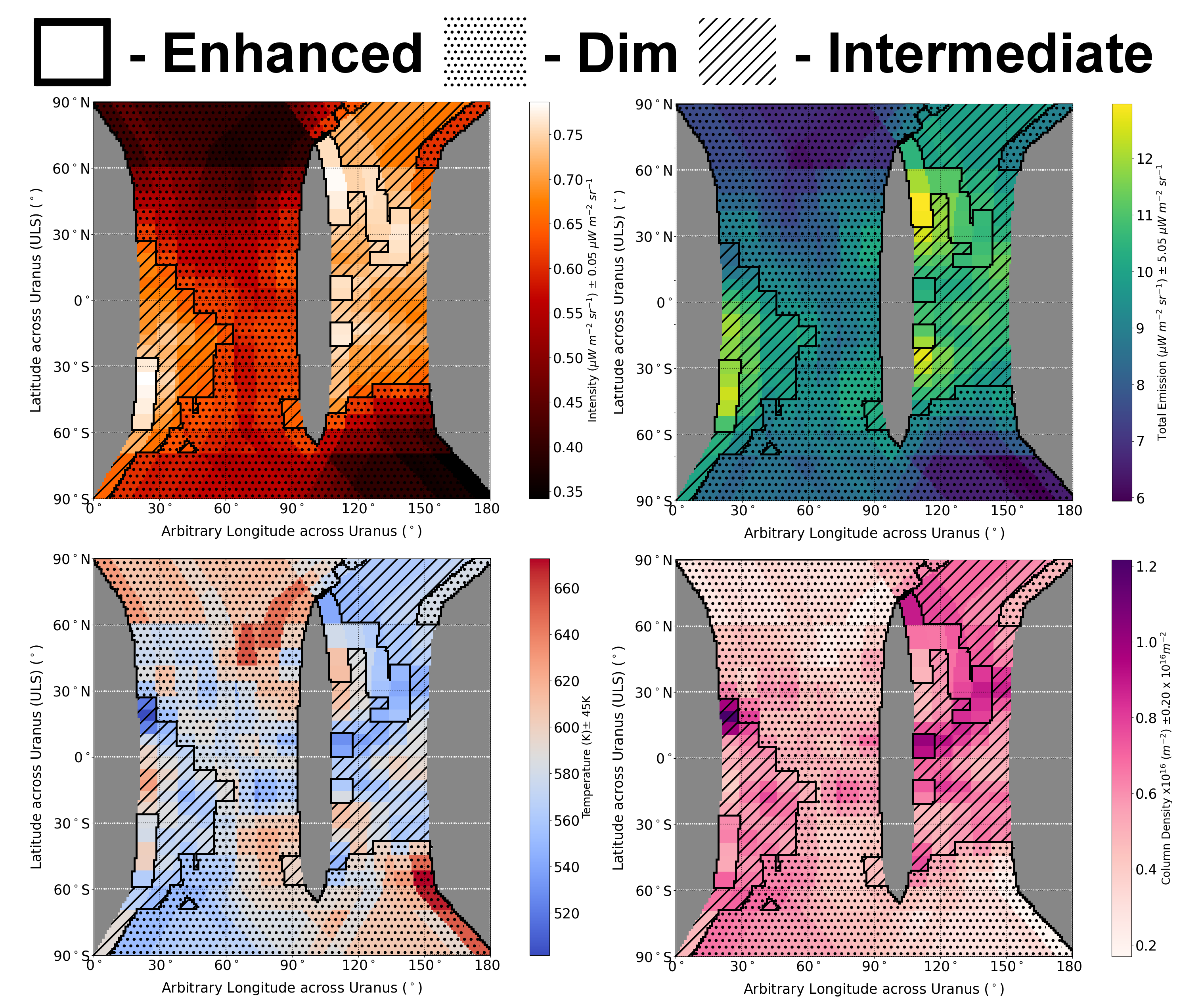
By Emma Thomas (University of Leicester)
Three decades of searching for the infrared aurorae finally come to a successful conclusion as portions of the northern (IAU southern) aurorae have been confirmed at Uranus. The icy planet represents an enigma within our solar system, with the first and only visit by Voyager II in 1986, it remains one of the least documented planets in our solar system. This is exceptionally apparent with the planet’s history of auroral observations, where the UV aurorae have been observed a handful of times but no infrared (IR) counterpart has been confirmed, despite both aurorae appearing at Jupiter and Saturn. Analysis of IR aurorae at both Jupiter and Saturn have challenged what we know about magnetosphere-ionosphere coupling, highlighting a need for IR analysis at Uranus to uncover its mysteries. Since 2020 our team has meticulously analysed archived data of Uranus during 2006 from the Keck II telescope on Mauna Kea in Hawai’i. The timing of these observations was key, close to equinox, as it provided an optimal view of the predicted locations of the northern and southern aurorae. By examining the emission lines from these aurorae (the emitting ion being H3+) between 3.94 to 4.01 μm, we carried out a full spectrum best fit across 5 fundamental lines for each spatial pixel across the planet’s disk. By comparing these lines at specific locations, we were able to identify an average 88% increase in column ion densities with no significant temperature changes localised close to or at expected auroral locations for the northern aurora. With this confirmation at Uranus, we look forward to a new age of auroral investigations at both ice giant planets.
References:
Thomas, E.M., Melin, H., Stallard, T.S. et al. Detection of the infrared aurora at Uranus with Keck-NIRSPEC. Nat Astron (2023). https://doi.org/10.1038/s41550-023-02096-5
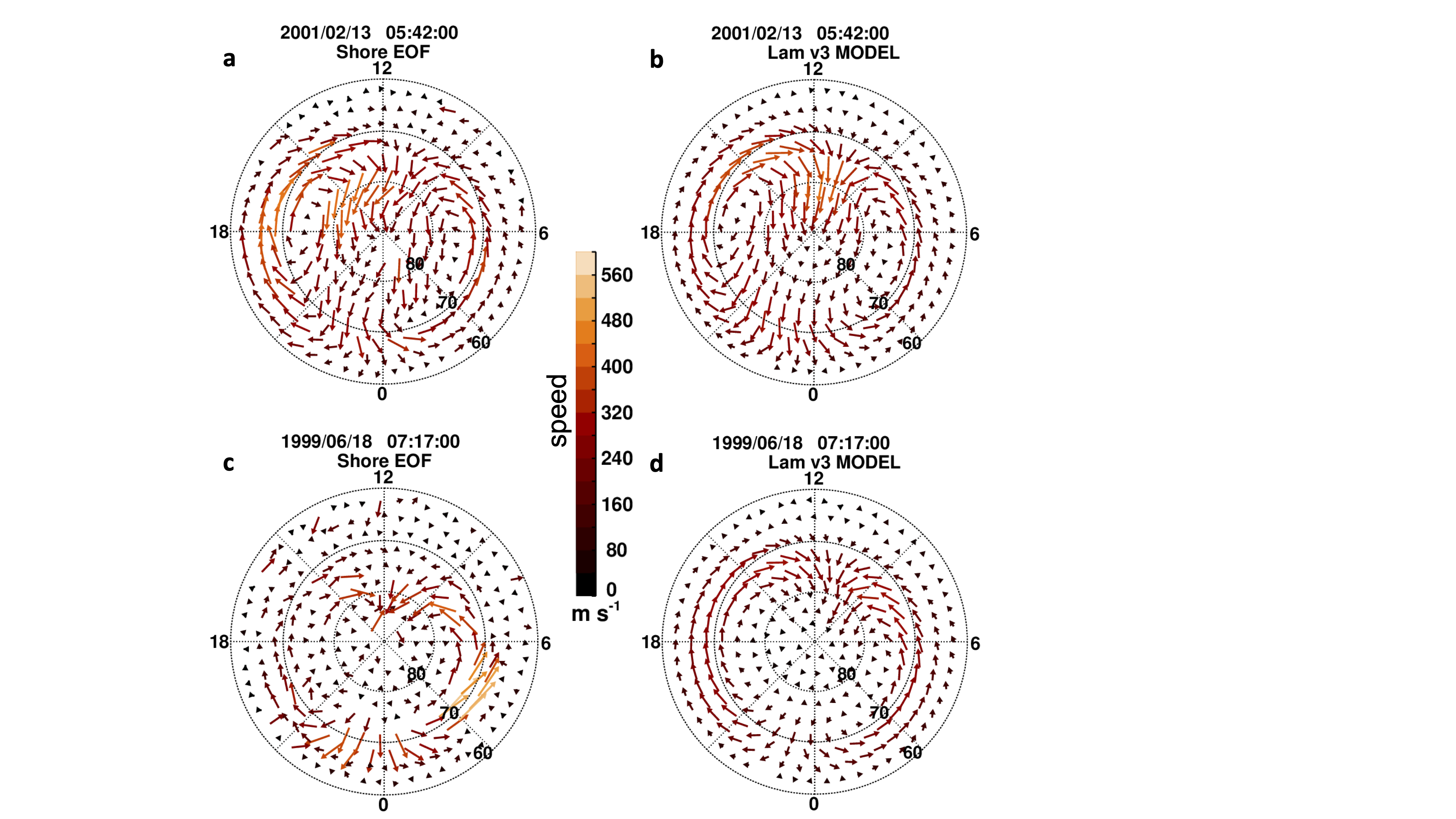
A Model of High Latitude Ionospheric Convection derived from SuperDARN radar EOF Data
By Mai Mai Lam (British Antarctic Survey)
Variations in space weather in the ionized region of the Earth’s atmosphere (the ionosphere) can result in expansion of the atmosphere, increasing the atmospheric drag on objects, such as satellites, in the thermosphere. We aim to significantly improve the forecasting of the effects of atmospheric drag on satellites by more accurate modelling of space weather effects on the motion of ionized particles (plasma) in the ionosphere. We have developed a model of the variation in plasma motion using a small number of solar wind variables. The model was built using a solar cycle’s worth (1997 to 2008 inclusive) of 5-minute resolution Empirical Orthogonal Function (EOF) patterns derived from Super Dual Auroral Radar Network (SuperDARN) line-of-sight observations of the plasma motion in the high-latitude northern hemisphere ionosphere (Shore et al., 2021). The model is driven by four variables: (1) the interplanetary magnetic field component By, (2) the solar wind coupling parameter epsilon, (3) a trigonometric function of the day-of-year, and (4) the monthly solar radio flux at 10.7 cm (the F10.7 index). Our model is good at reproducing the original data set - if 0 indicates that there is no reproduction and 1 indicates exact reproduction, then our model scores 0.7. Data set reproduction is best around the maximum in the solar cycle and worst at solar minimum. This is mainly due to differences in the spatiotemporal data coverage between these times but possibly also due to the model’s specification of the physical processes coupling the Sun to the Earth’s ionosphere. Our model could easily be used to forecast the ionospheric electric field about 1 hour in advance, using the real-time solar wind data available from spacecraft located upstream of the Earth.
References:
Lam, M. M., Shore, R. M., Chisham, G., Freeman, M. P., Grocott, A., Walach, M.-T., & Orr, L. (2023). A model of high latitude ionospheric convection derived from SuperDARN EOF model data. Space Weather, 21, e2023SW003428. https://doi.org/10.1029/2023SW003428
Shore, R. M., Freeman, M., Chisham, G., Lam, M. M., & Breen, P. (2022). Dominant spatial and temporal patterns of horizontal ionospheric plasma velocity variation covering the northern polar region, from 1997.0 to 2009.0 - VERSION 2.0 (Version 2.0) [Dataset]. NERC EDS UK Polar Data Centre. https://doi.org/10.5285/2b9f0e9f-34ec-4467-9e02-abc771070cd9