MIST
Magnetosphere, Ionosphere and Solar-Terrestrial
Latest articles
- Temporal Variability of Saturn's H2 Dayglow and Northern Aurora Observed by Hisaki and Cassini
- The Jupiter Auroral Ionosphere Code
- Analysis of Chorus Wave Power on Burst‐Mode Timescales During the Van Allen Probes Era
- Soft X-Ray Emission from Saturn's Magnetosheath II: Solar Wind Driving
- Which Kelvin-Helmholtz waves grow along the spatially-varying magnetopause flanks and why?
Latest news
Open Letter Ready For Signatories
Protect MIST Science! Sign the MIST Community Open Letter on the STFC funding cuts!
https://sites.google.com/view/uk-mist-community-open-letter
Statement from MIST Council regarding the STFC Funding Situation
Statement from MIST Council regarding the STFC Funding Situation
MIST Council is deeply concerned by the ongoing STFC funding uncertainty and its impact on our community and beyond.
The current combination of prospective delayed and reduced funding, together with already volatile financial situations at universities across the UK, is placing significant strain on research groups. In some cases, institutions may be unable to support researchers through gaps between projects, increasing precarity across the community and adding significant pressure on early-career researchers.
We are concerned that continued uncertainty risks accelerating a brain drain from the UK, as skilled researchers reconsider their future in a system offering limited stability. The loss of expertise at any career stage would have lasting consequences for UK space science.
What is going on?
For those that are unaware of the situation, it is complex and evolving. We suggest the following sources to get up to speed on the current developments.
https://ras.ac.uk/news-and-press/news/proposed-budget-cuts-catastrophe-uk-astronomy
What are we doing about it?
Behind the scenes, MIST Council is actively engaging with relevant parties to understand the scale of the challenge and to identify constructive ways forward.
- We are seeking seasoned members of the community to join MIST Council on a task force to help develop options and represent the needs of our community. If you would like to be involved, please reach out to us via the MIST Council email (This email address is being protected from spambots. You need JavaScript enabled to view it.) by the end of this week (13th February 2026).
- In addition to the task force, we want to provide an open forum for discussion and collective input among all members of the wider MIST community. We are exploring options and will be in touch as soon as possible with further details.
- We believe in working together in the face of the current challenges and we are collaborating with UKSP and others to strive for a fair and positive outcome for all. We are reaching out to members of the SSAP (Solar System Advisory Panel) to explore the hosting of a community town hall meeting, like the one already being organised by the AAP (Astronomy Advisory Panel), to provide an open forum for discussion and collective input.
What can you do to help?
There are several open letters representing people in various career stages that have been made available to sign. We encourage you to read the relevant letter(s) and to sign them if you support them:
- Fellowship Holders: https://advancedfellows-openletter-stfc.github.io/index.html
- Early Career Researchers: https://ecr-openletter-stfc.github.io/
The Royal Astronomical Society are also urging Fellows to lobby their MPs against the cuts, and have included a template letter that can be used to do so:
https://ras.ac.uk/news-and-press/news/ras-fellows-urged-lobby-against-unprecedented-cuts
MIST Council will continue to advocate for transparency, stability, and funding structures that recognise both the long-term nature of our science and the people who deliver it.
We thank you for your continued support in this period of uncertainty.
Please contact This email address is being protected from spambots. You need JavaScript enabled to view it. if you have further suggestions.
MIST Council
![]()
Announcement of New MIST Council 2025
We are very pleased to announce the following members of the community have been elected to MIST Council:
- Gemma Bower (University of Leicester), MIST Councillor
- Tom Elsden (University of St Andrews), MIST Councillor
- Cameron Patterson (Lancaster University), MIST Councillor
- Fiona Ball (University of Southampton), Student Representative
They will begin their terms in July 2025.
We thank outgoing MIST Council members: Maria Walach, Chiara Lazzeri and Emma Woodfield. Andy Smith will remain on council a little longer as a co-opted member to cover Rosie Johnson's maternity leave.
The current composition of Council can be found on our website (https://www.mist.ac.uk/community/mist-council).
Announcement of New MIST Councillors.
We are very pleased to announce the following members of the community have been elected unopposed to MIST Council:
- Rosie Johnson (Aberystwyth University), MIST Councillor
- Matthew Brown (University of Birmingham), MIST Councillor
- Chiara Lazzeri (MSSL, UCL), Student Representative
Rosie, Matthew, and Chiara will begin their terms in July. This will coincide with Jasmine Kaur Sandhu, Beatriz Sanchez-Cano, and Sophie Maguire outgoing as Councillors.
The current composition of Council can be found on our website, and this will be amended in July to reflect this announcement (https://www.mist.ac.uk/community/mist-council).
Nominations are open for MIST Council
We are very pleased to open nominations for MIST Council. There are three positions available (detailed below), and elected candidates would join Georgios Nicolaou, Andy Smith, Maria-Theresia Walach, and Emma Woodfield on Council. The nomination deadline is Friday 31 May.
Council positions open for nomination
2 x MIST Councillor - a three year term (2024 - 2027). Everyone is eligible.
MIST Student Representative - a one year term (2024 - 2025). Only PhD students are eligible. See below for further details.
About being on MIST Council
If you would like to find out more about being on Council and what it can involve, please feel free to email any of us (email contacts below) with any of your informal enquiries! You can also find out more about MIST activities at mist.ac.uk. Two of our outgoing councillors, Beatriz and Sophie, have summarised their experiences being on MIST Council below.
Beatriz Sanchez-Cano (MIST Councillor):
"Being part of the MIST council for the last 3 years has been a great experience personally and professionally, in which I had the opportunity to know better our community and gain a larger perspective of the matters that are important for the MIST science progress in the UK. During this time, I’ve participated in a number of activities and discussions, such as organising the monthly MIST seminars, Autumn MIST meetings, writing A&G articles, and more importantly, being there to support and advise our colleagues in cases of need together with the wonderful council members. MIST is a vibrant and growing community, and the council is a faithful reflection of it."
Sophie Maguire (MIST Student Representative):
"Being the student representative for MIST council has been an amazing experience. I have been part of organizing conferences, chairing sessions, and writing grant applications based on the feedback MIST has received. From a wider perspective, MIST has helped to grow and support my professional networks which in turn, directly benefits my PhD work as well. I would encourage any PhD student to apply for the role of MIST Student Representative and I would be happy to answer any questions or queries you have about the role."
How to nominate
If you would like to stand for election or you are nominating someone else (with their agreement!) please email This email address is being protected from spambots. You need JavaScript enabled to view it. by Friday 31 May. If there is a surplus of nominations for a role, then an online vote will be carried out with the community. Please include the following details in the nomination:
- Name
- Position (Councillor/Student Rep.)
- Nomination Statement (150 words max including a bit about the nominee and focusing on your reasons for nominating. This will be circulated to the community in the event of a vote.)
MIST Council details
- Sophie Maguire, University of Birmingham, Earth's ionosphere - This email address is being protected from spambots. You need JavaScript enabled to view it.
- Georgios Nicolaou, MSSL, solar wind plasma - This email address is being protected from spambots. You need JavaScript enabled to view it.
- Beatriz Sanchez-Cano, University of Leicester, Mars plasma - This email address is being protected from spambots. You need JavaScript enabled to view it.
- Jasmine Kaur Sandhu, University of Leicester, Earth’s inner magnetosphere - This email address is being protected from spambots. You need JavaScript enabled to view it.
- Andy Smith, Northumbria University, Space Weather - This email address is being protected from spambots. You need JavaScript enabled to view it.
- Maria-Theresia Walach, Lancaster University, Earth’s ionosphere - This email address is being protected from spambots. You need JavaScript enabled to view it.
- Emma Woodfield, British Antarctic Survey, radiation belts - This email address is being protected from spambots. You need JavaScript enabled to view it.
- MIST Council email - This email address is being protected from spambots. You need JavaScript enabled to view it.
Nuggets of MIST science, summarising recent papers from the UK MIST community in a bitesize format.
If you would like to submit a nugget, please fill in the following form: https://forms.gle/Pn3mL73kHLn4VEZ66 and we will arrange a slot for you in the schedule. Nuggets should be 100–300 words long and include a figure/animation. Please get in touch!
If you have any issues with the form, please contact This email address is being protected from spambots. You need JavaScript enabled to view it..
Temporal Variability of Saturn's H2 Dayglow and Northern Aurora Observed by Hisaki and Cassini
Temporal Variability of Saturn's H2 Dayglow and Northern Aurora Observed by Hisaki and Cassini
By Leah Clare (Lancaster University)
The ultraviolet (UV) emissions from Saturn are composed of the dayglow from the sunlit atmosphere and the aurorae at the poles. Investigation into the daily variability of the dayglow remains somewhat unconstrained, particularly on timescales of weeks. Utilising coincident Hisaki and Cassini observations across ~3 weeks in 2014, we determine the temporal variability of the UV emitted power, assess the response of the dayglow to solar activity, and constrain the contribution from the northern aurora to the total emitted power. We find that the power varies by a factor of 2.26 over 23 days with Hisaki, and 1.29 over 17 days with Cassini. Upon separation of the northern auroral contribution with Cassini, the contribution is found to be between 10% - 26%. Additionally, the dayglow component displays a strong correlation with solar activity, confirming that the dayglow is controlled by the UV solar flux as shown by previous studies (Gustin et al., 2010; Liu & Dalgarno 1996). This study demonstrates the first analysis of the Saturn campaigns by Hisaki, allowing an assessment of the robustness of such a mission in observing outer planet targets. The multi-mission analysis confirmed that Hisaki was able to track the variability of the UV emissions from Saturn, with comparative trends to the Cassini data.
References:
Gustin, J., Stewart, I., Gérard, J. C., & Esposito, L. (2010). Characteristics of Saturn’s FUV airglow from limb-viewing spectra obtained with Cassini-UVIS. Icarus, 210(1), 270–283. https://doi.org/10.1016/j.icarus.2010.06.031
Liu, W., & Dalgarno, A. (1996). The Ultraviolet Spectrum of the Jovian Dayglow. The Astrophysical Journal, (462), 502–518.
See publication for more details:
https://doi.org/10.1029/2026JA035194
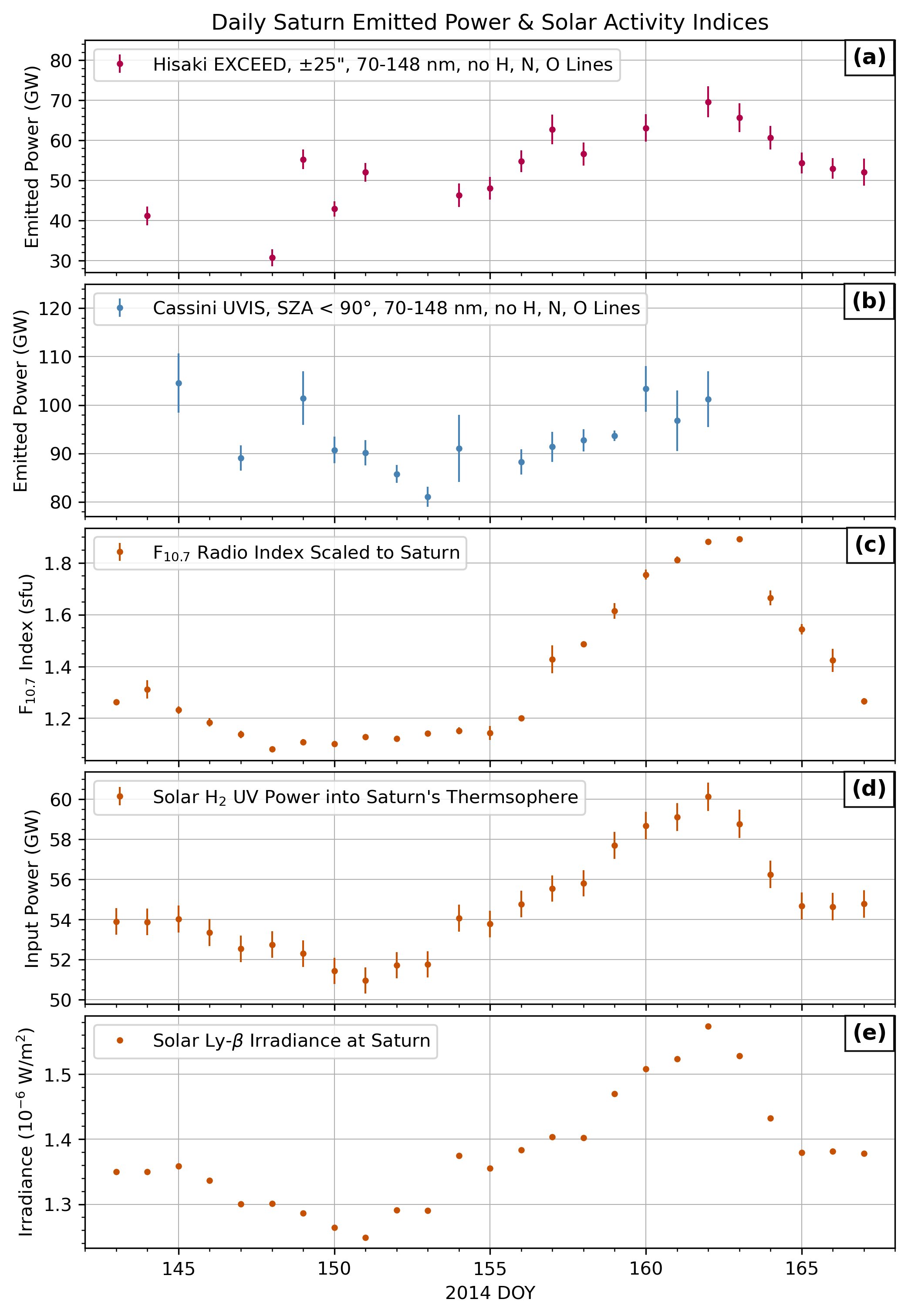
(a) The total emitted UV power obtained from Hisaki/EXCEED. The points are daily average H2 powers from 70 to 148 nm. (b) The total emitted UV power determined with Cassini UVIS; each point is the daily average H2 power for the wavelength range 70–148 nm. (c) The daily average solar F10.7 radio index, a proxy for EUV radiation, scaled to Saturn. Data from Space Weather Canada. (d) The solar EUV power into Saturn's thermosphere. Solar spectral irradiance data are obtained from LISIRD, which uses the Flare Solar Irradiance Model (Chamberlin et al., 2008) and Earth irradiance measurements. The calculation is from Gershman and DiBraccio (2024). (e) The solar H‐Lyman β irradiance at Saturn; data are obtained from LISIRD, which uses the Flare Solar Irradiance Model (Chamberlin et al., 2008) and Earth irradiance measurements.
Solar Activity References:
Chamberlin, P. C., Woods, T. N., & Eparvier, F. G. (2008). Flare irradiance spectral model (fism): Flare component algorithms and results. Space Weather, 6(5). https://doi.org/10.1029/2007SW000372
Gershman, D. J., & DiBraccio, G. A. (2024). Quantifying External Energy Inputs for Giant Planet Magnetospheres. Geophysical Research Letters, 51(15). https://doi.org/10.1029/2024GL109660
The Jupiter Auroral Ionosphere Code
The Jupiter Auroral Ionosphere Code
By Jonathan Nichols (University of Leicester)
We present a new model of auroral precipitation and associated phenomena at Jupiter, called the Jupiter Auroral Ionosphere Code (JAIC). The hybrid model follows the primary electron population using a Monte Carlo code that runs on a GPU, and computes the contribution of the secondaries using a two‐stream approximation. The model includes modules that compute high resolution far‐ultraviolet H2 spectra, the H3+ density using simple ion chemistry, and the resulting Pedersen conductivity and H3+ radiance. We illustrate the validity of the model and present a number of initial applications. We show that the model successfully relates Juno auroral electron and UV observations, and that an auroral polar transient form is consistent with excitation by ∼ 23± 4 keV electrons. We also compute a self‐consistent relation between field‐aligned current density and Pedersen conductance and show that it is consistent with Juno in situ observations. We suggest that Joule heating enabled by the electron contribution to the Pedersen conductivity may explain heating observed at mbar levels. We further show that, in contrast with initial analysis, polar H3+ emissions observed by the James Webb Space Telescope are consistent with the electron population above the auroral zone.
The model is publicly available at GitHub and Zenodo: https://github.com/jdnplanets/jaic
See publication for more details:
Nichols, J. D. (2026). Jupiter's auroral ionosphere: Hybrid Monte Carlo, auroral spectrum and conductivity modeling. Journal of Geophysical Research: Space Physics, 131, e2026JA035228. https://doi.org/10.1029/2026JA035228
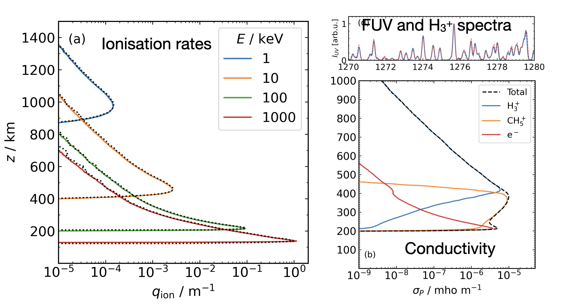
A selection of outputs from JAIC: ionisation rates, Pedersen conductivity and FUV spectra. For further details see Nichols (2026).
Analysis of Chorus Wave Power on Burst‐Mode Timescales During the Van Allen Probes Era
Analysis of Chorus Wave Power on Burst‐Mode Timescales During the Van Allen Probes Era
By Rachel Black (University of Exeter/British Antarctic Survey)
Interactions between whistler‐mode chorus waves and electrons are a key driver of dynamics in Earth’s radiation belts. These global dynamics are often described using Fokker‐Planck diffusion models. Whilst, in many cases, such models effectively describe the large scale changes within the region, they often rely upon spatially and temporally averaged representations of the wave properties. However, observations have shown that whistler‐mode chorus can display large sub‐second powers that challenge model assumptions and potentially give rise to non‐diffusive processes.
In this work, we investigate the power of whistler‐mode chorus on sub‐second timescales using the high‐resolution data capture mode on the Van Allen Probes’ Electric and Magnetic Field Instrument Suite and Integrated Science (EMFISIS). We show that peak chorus power on sub‐second timescales is regularly larger than the corresponding spacecraft “survey” power by over a factor of 100. The work also explores the magnetospheric conditions under which the largest sub‐second power variability of chorus waves is observed, and we find that trends vary across different chorus frequency bands. Notably, the largest powers are observed in the lower‐band frequency range during active conditions and between 21:00–12:00 MLT, where >46% of burst samples contain an instantaneous wave intensity that exceeds 2.25 × 10⁴ pT2. Further, binning the lower‐band power by the ratio of plasma‐to‐gyrofrequency separates the waves into two distinct low and high variability populations. The results quantify sub‐second wave power variability that may influence energetic electron dynamics not currently captured in time‐averaged wave models.
See publication for more details:
Black, R., Allanson, O., Meredith, N. P., Hillier, A., & Hartley, D. P. (2026). Analysis of chorus wave power on burst-mode timescales during the Van Allen Probes era. Journal of Geophysical Research: Space Physics, 131, e2026JA035082. https://doi.org/10.1029/2026JA035082

Chorus-containing records in the burst-mode measurements from the Van Allen Probes' EMFISIS instruments when at equatorial latitudes ($|\lambda_m|<$6.$^\circ$). Chorus emissions are divided into low frequency, lower-band and upper-band frequency ranges. For each frequency range, the subpanels show (a)-(c) average chorus power for corresponding survey-mode events; (d)-(f) maximum chorus power from burst-mode events; (g)-(i) ratio between the maximum burst power and the survey power; and (j)-(l) the normalized inter-quartile range ($\frac{Q3-Q1}{Q2}$) for each burst record.
Soft X-Ray Emission from Saturn's Magnetosheath II: Solar Wind Driving
Soft X-Ray Emission from Saturn's Magnetosheath II: Solar Wind Driving
By Dan Naylor (Lancaster University)
Saturn’s magnetosphere is dominated by Enceladus-sourced, water-group neutrals that form a torus and extend into the magnetosheath. Soft X-ray emission can be generated in the magnetosheath due to charge exchange between highly charged solar wind ions and the neutrals. Imaging of the soft X-rays is an emerging technology that aims to provide a more global and dynamic view of the magnetosheath and, for example, give insights into the driving of the magnetosphere by the solar wind. The ESA/CAS SMILE mission has now launched and aims to image the terrestrial magnetosheath. We, along with Rogan et al. (2026, https://doi.org/10.1029/2025JA034462), explore the viability of soft X-ray imaging at Saturn. We consider charge exchange between Enceladus-sourced H, O and OH and solar wind ions O7+ and O8+ to estimate the emission rates from the system and the flux detected by a soft X-ray imager (SXI) at the system. We also vary solar wind dynamic pressure to test the effect of changing solar wind conditions on X-ray production. X-ray volumetric emission rate is on the order of 10-11 to 10-10 photon cm-3 s-1 for slow and fast solar winds. For a SMILE-like SXI imaging the system from around 50 RS, >100 photons could be detected within a quarter of a planetary rotation. A hypothetical future instrument with increased FOV and effective area significantly increases photon count rate, highlighting that X-ray imaging may be a useful technique to better understand Saturn’s magnetosphere and neutral environment on a potential future mission.
See publication for more details:
Naylor, D., Ray, L. C., Rogan, P. C., Dunn, W. R., & Smith, H. T. (2026). Soft X-ray emission from Saturn's magnetosheath II: Solar wind driving. Journal of Geophysical Research: Space Physics, 131, e2025JA034461. https://doi.org/10.1029/2025JA034461
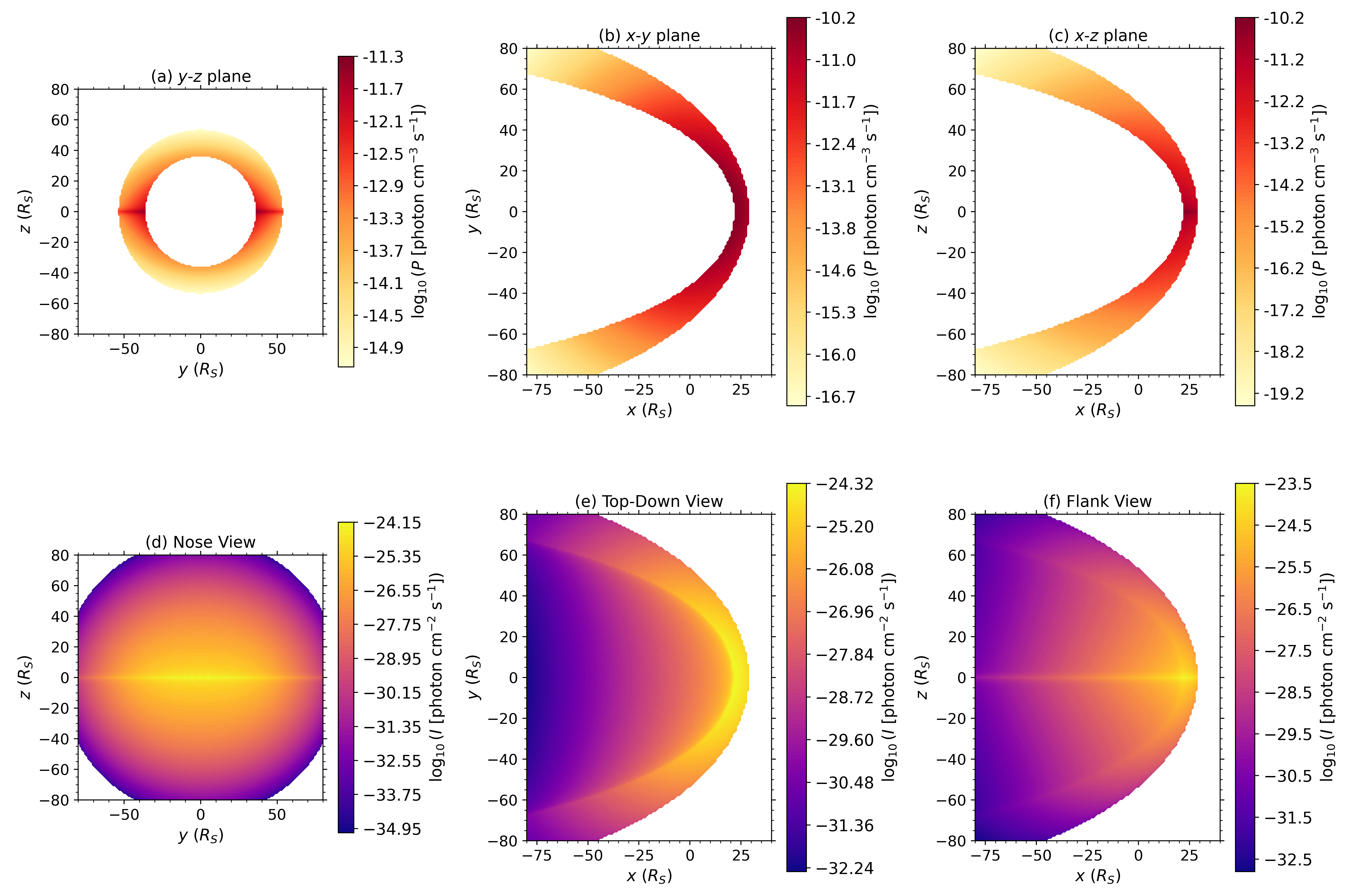
Emission rate slices (a, b, c) in the y-z, x-y and x-z planes and modelled intensity maps (d, e, f) for a nose-on, top-down and side-on view of the system, for a SMILE-like soft X-ray imager at ~50 RS from Saturn.
Which Kelvin-Helmholtz waves grow along the spatially-varying magnetopause flanks and why?
Which Kelvin-Helmholtz waves grow along the spatially-varying magnetopause flanks and why?
By Harley Kelly (Imperial College London)
The Kelvin-Helmholtz instability mediates the viscous-like solar-terrestrial interaction, allowing solar wind plasma and energy to penetrate our magnetic shield through generating magnetopause surface waves that quickly become non-linear. Determining when and where this should occur and which wave modes grow has remained challenging. This is because the underlying theory has concentrated on local wave growth, where the locally most-unstable linear wave dominates. However, these waves travel along the boundary into new regions where the instability is still able to amplify these perturbations despite the different background properties. Two possible paradigms exist, waves are either:
(a) locally generated, being those predicted by the simple theory
(b) originate further upstream, having travelled and grown along the way
We address this conundrum by applying a machine learning technique, Dynamic Mode Decomposition, that efficiently extracts distinct wave modes from a simulation of the entire magnetosphere. This shows Kelvin-Helmholtz waves do grow quickly out of some points on the boundary, signaling local generation. However, their energy persists as they travel down the tail, slowly growing in both amplitude and spatial extent in the process due to the accelerating flow around the magnetosphere and its effect on the instability. Therefore, both effects play a role in which waves are dominant at any point.
These results may explain why longer wavelengths are observed in the tail than local theory predicts and motivates further exploration of tangential inhomogeneities in basic Kelvin-Helmholtz theory. We also highlight that Dynamic Mode Decomposition may prove a powerful technique for studying other forms of waves, instabilities and turbulence across the heliosphere.
See publication for more details:
Kelly, H. M., Archer, M. O., Eastwood, J. P., Heyns, M., Eggington, J. W. B. and Chittenden, J. P (2026). Superposition of Doppler-Shifting Magnetopause Kelvin-Helmholtz Modes Through Dynamic Mode Decomposition of a Global MHD Simulation. Geophysical Research Letters, 53, e2025GL120284, https://doi.org/10.1029/2025GL120284
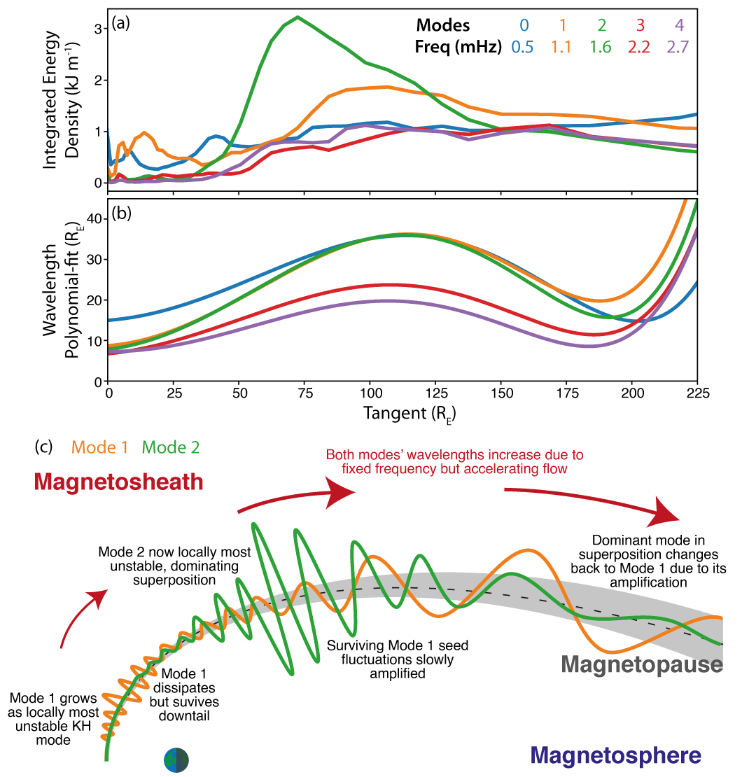
Comparison of dynamic mode decomposition modes along equatorial magnetopause tangent showing (a) integrated energy densities and (b) polynomial-fit wavelengths. (c) Cartoon depicting key results.