MIST
Magnetosphere, Ionosphere and Solar-Terrestrial
Latest articles
- Temporal Variability of Saturn's H2 Dayglow and Northern Aurora Observed by Hisaki and Cassini
- The Jupiter Auroral Ionosphere Code
- Analysis of Chorus Wave Power on Burst‐Mode Timescales During the Van Allen Probes Era
- Soft X-Ray Emission from Saturn's Magnetosheath II: Solar Wind Driving
- Which Kelvin-Helmholtz waves grow along the spatially-varying magnetopause flanks and why?
Latest news
Open Letter Ready For Signatories
Protect MIST Science! Sign the MIST Community Open Letter on the STFC funding cuts!
https://sites.google.com/view/uk-mist-community-open-letter
Statement from MIST Council regarding the STFC Funding Situation
Statement from MIST Council regarding the STFC Funding Situation
MIST Council is deeply concerned by the ongoing STFC funding uncertainty and its impact on our community and beyond.
The current combination of prospective delayed and reduced funding, together with already volatile financial situations at universities across the UK, is placing significant strain on research groups. In some cases, institutions may be unable to support researchers through gaps between projects, increasing precarity across the community and adding significant pressure on early-career researchers.
We are concerned that continued uncertainty risks accelerating a brain drain from the UK, as skilled researchers reconsider their future in a system offering limited stability. The loss of expertise at any career stage would have lasting consequences for UK space science.
What is going on?
For those that are unaware of the situation, it is complex and evolving. We suggest the following sources to get up to speed on the current developments.
https://ras.ac.uk/news-and-press/news/proposed-budget-cuts-catastrophe-uk-astronomy
What are we doing about it?
Behind the scenes, MIST Council is actively engaging with relevant parties to understand the scale of the challenge and to identify constructive ways forward.
- We are seeking seasoned members of the community to join MIST Council on a task force to help develop options and represent the needs of our community. If you would like to be involved, please reach out to us via the MIST Council email (This email address is being protected from spambots. You need JavaScript enabled to view it.) by the end of this week (13th February 2026).
- In addition to the task force, we want to provide an open forum for discussion and collective input among all members of the wider MIST community. We are exploring options and will be in touch as soon as possible with further details.
- We believe in working together in the face of the current challenges and we are collaborating with UKSP and others to strive for a fair and positive outcome for all. We are reaching out to members of the SSAP (Solar System Advisory Panel) to explore the hosting of a community town hall meeting, like the one already being organised by the AAP (Astronomy Advisory Panel), to provide an open forum for discussion and collective input.
What can you do to help?
There are several open letters representing people in various career stages that have been made available to sign. We encourage you to read the relevant letter(s) and to sign them if you support them:
- Fellowship Holders: https://advancedfellows-openletter-stfc.github.io/index.html
- Early Career Researchers: https://ecr-openletter-stfc.github.io/
The Royal Astronomical Society are also urging Fellows to lobby their MPs against the cuts, and have included a template letter that can be used to do so:
https://ras.ac.uk/news-and-press/news/ras-fellows-urged-lobby-against-unprecedented-cuts
MIST Council will continue to advocate for transparency, stability, and funding structures that recognise both the long-term nature of our science and the people who deliver it.
We thank you for your continued support in this period of uncertainty.
Please contact This email address is being protected from spambots. You need JavaScript enabled to view it. if you have further suggestions.
MIST Council
![]()
Announcement of New MIST Council 2025
We are very pleased to announce the following members of the community have been elected to MIST Council:
- Gemma Bower (University of Leicester), MIST Councillor
- Tom Elsden (University of St Andrews), MIST Councillor
- Cameron Patterson (Lancaster University), MIST Councillor
- Fiona Ball (University of Southampton), Student Representative
They will begin their terms in July 2025.
We thank outgoing MIST Council members: Maria Walach, Chiara Lazzeri and Emma Woodfield. Andy Smith will remain on council a little longer as a co-opted member to cover Rosie Johnson's maternity leave.
The current composition of Council can be found on our website (https://www.mist.ac.uk/community/mist-council).
Announcement of New MIST Councillors.
We are very pleased to announce the following members of the community have been elected unopposed to MIST Council:
- Rosie Johnson (Aberystwyth University), MIST Councillor
- Matthew Brown (University of Birmingham), MIST Councillor
- Chiara Lazzeri (MSSL, UCL), Student Representative
Rosie, Matthew, and Chiara will begin their terms in July. This will coincide with Jasmine Kaur Sandhu, Beatriz Sanchez-Cano, and Sophie Maguire outgoing as Councillors.
The current composition of Council can be found on our website, and this will be amended in July to reflect this announcement (https://www.mist.ac.uk/community/mist-council).
Nominations are open for MIST Council
We are very pleased to open nominations for MIST Council. There are three positions available (detailed below), and elected candidates would join Georgios Nicolaou, Andy Smith, Maria-Theresia Walach, and Emma Woodfield on Council. The nomination deadline is Friday 31 May.
Council positions open for nomination
2 x MIST Councillor - a three year term (2024 - 2027). Everyone is eligible.
MIST Student Representative - a one year term (2024 - 2025). Only PhD students are eligible. See below for further details.
About being on MIST Council
If you would like to find out more about being on Council and what it can involve, please feel free to email any of us (email contacts below) with any of your informal enquiries! You can also find out more about MIST activities at mist.ac.uk. Two of our outgoing councillors, Beatriz and Sophie, have summarised their experiences being on MIST Council below.
Beatriz Sanchez-Cano (MIST Councillor):
"Being part of the MIST council for the last 3 years has been a great experience personally and professionally, in which I had the opportunity to know better our community and gain a larger perspective of the matters that are important for the MIST science progress in the UK. During this time, I’ve participated in a number of activities and discussions, such as organising the monthly MIST seminars, Autumn MIST meetings, writing A&G articles, and more importantly, being there to support and advise our colleagues in cases of need together with the wonderful council members. MIST is a vibrant and growing community, and the council is a faithful reflection of it."
Sophie Maguire (MIST Student Representative):
"Being the student representative for MIST council has been an amazing experience. I have been part of organizing conferences, chairing sessions, and writing grant applications based on the feedback MIST has received. From a wider perspective, MIST has helped to grow and support my professional networks which in turn, directly benefits my PhD work as well. I would encourage any PhD student to apply for the role of MIST Student Representative and I would be happy to answer any questions or queries you have about the role."
How to nominate
If you would like to stand for election or you are nominating someone else (with their agreement!) please email This email address is being protected from spambots. You need JavaScript enabled to view it. by Friday 31 May. If there is a surplus of nominations for a role, then an online vote will be carried out with the community. Please include the following details in the nomination:
- Name
- Position (Councillor/Student Rep.)
- Nomination Statement (150 words max including a bit about the nominee and focusing on your reasons for nominating. This will be circulated to the community in the event of a vote.)
MIST Council details
- Sophie Maguire, University of Birmingham, Earth's ionosphere - This email address is being protected from spambots. You need JavaScript enabled to view it.
- Georgios Nicolaou, MSSL, solar wind plasma - This email address is being protected from spambots. You need JavaScript enabled to view it.
- Beatriz Sanchez-Cano, University of Leicester, Mars plasma - This email address is being protected from spambots. You need JavaScript enabled to view it.
- Jasmine Kaur Sandhu, University of Leicester, Earth’s inner magnetosphere - This email address is being protected from spambots. You need JavaScript enabled to view it.
- Andy Smith, Northumbria University, Space Weather - This email address is being protected from spambots. You need JavaScript enabled to view it.
- Maria-Theresia Walach, Lancaster University, Earth’s ionosphere - This email address is being protected from spambots. You need JavaScript enabled to view it.
- Emma Woodfield, British Antarctic Survey, radiation belts - This email address is being protected from spambots. You need JavaScript enabled to view it.
- MIST Council email - This email address is being protected from spambots. You need JavaScript enabled to view it.
Nuggets of MIST science, summarising recent papers from the UK MIST community in a bitesize format.
If you would like to submit a nugget, please fill in the following form: https://forms.gle/Pn3mL73kHLn4VEZ66 and we will arrange a slot for you in the schedule. Nuggets should be 100–300 words long and include a figure/animation. Please get in touch!
If you have any issues with the form, please contact This email address is being protected from spambots. You need JavaScript enabled to view it..
Timescales of Birkeland Currents Driven by the IMF
By John Coxon (University of Southampton)
Birkeland currents are the mechanism by which information is communicated from Earth’s magnetopause to the ionosphere. Understanding the timescales of these currents is very useful for understanding the ionosphere’s reaction to magnetopause phenomena. We use the Active Magnetosphere and Planetary Electrodynamics Response Experiment (AMPERE) dataset, which uses magnetometers on 66 spacecraft in low Earth orbit to derive Birkeland current density on a grid of colatitude and magnetic local time. The current densities are derived in a ten minute sliding window, evaluated every two minutes.
We use the SPatial Information from Distributed Exogenous Regression (SPIDER) technique (Shore et al, 2019), which treats each coordinate of a global dataset (e.g. AMPERE or SuperMAG) independently, regressing the time series in each coordinate against some external driver to find the time lag that maximises the correlation of the two.
The figure below shows the correlation (left) and lag (centre) of the current densities with Interplanetary Magnetic Field (IMF) Bz. We focus on the R1 and R2 regions (right) here. Southward (negative) Bz drives Birkeland current as a result of magnetic reconnection, as shown by the correlations. Looking at the lags on the dayside, the poleward lags are 10–20 minutes, reflecting the time taken for the Birkeland currents to start to react to magnetic reconnection. At all MLT, the equatorward lags are 60–90 minutes, reflecting the time at which the polar cap is largest. On the nightside, the poleward lags are 90–150 minutes, reflecting how long it takes the polar cap to contract during nightside reconnection. More details on the R1/R2 correlations, and other correlations between Birkeland current and IMF Bz and By, are available in the full study.
For more information, please see the paper:
, , , , , , et al. ( 2019). Timescales of Birkeland currents driven by the IMF. Geophysical Research Letters, 46, 7893– 7901. https://doi.org/10.1029/2018GL081658

Figure: Correlation (left) and lag (centre) of AMPERE current density with IMF Bz in March 2010. A key to the regions visible is presented in the right-hand panel, to allow easy references in the text above.
The Impact of Radiation Belt Enhancements on Electric Orbit Raising
By Alexander Lozinski (British Antarctic Survey)
Electric orbit raising is a method of getting satellites into geostationary orbit (GEO) using low-thrust electric propulsion. A satellite intended for GEO is first placed into elliptical geostationary transfer orbit after separating from the launch vehicle. Following this, maneuvers are performed to raise the satellite to GEO. In conventional launches, chemical propulsion is used and this process requires a few days. With electrical thrusters, orbit raising can be performed more efficiently but requires a longer period (around 200 days) due to the lower thrust.
This method of raising satellites was introduced commercially in 2014 with the launch of the first all-electric satellites. Although the lower wet mass due to lack of chemical propellant reduces launch costs, the longer time required for the satellite to reach GEO leaves it exposed to irradiation from trapped protons of the Van Allen belts. This can cause degradation to solar cells via non-ionising displacement collisions.
Sustained enhancements in trapped proton flux can occur via trapping of solar energetic particles following a large geomagnetic disturbance. In this work, the solar cell degradation through time for a variety of real electric orbit raising scenarios was calculated in both a quiet and active environment, based on measurements taken by CRRES before/after the March 1991 storm. The trajectories of two previously launched satellites (EOR-1 and EOR-2) that underwent electric orbit raising is shown in the figure. The figure also shows the calculated remaining output power of the solar cell, P/P0, through time for both trajectories in an active environment. Reductions in P/P0 represent degradation to the solar cells.
A key finding is a large (up to 5%) increase in P/P0 degradation that occurs when electric orbit raising is performed in an enhanced radiation belt environment. However, the figure also demonstrates that some orbits are more at risk than others. Orbits with a higher initial apogee (e.g. EOR-2, red line) spend less time in regions of high proton flux, and experience less degradation. The work highlights the significant impacts of an enhanced environment on solar cell degradation, and identifies how this degradation can in part be mitigated with an appropriate choice of orbit and shielding.
For more information, please see the paper:
Lozinski, A. R., Horne, R. B., Glauert, S. A., Del Zanna, G., Heynderickx, D., & Evans, H. D. R. ( 2019). Solar cell degradation due to proton belt enhancements during electric orbit raising to GEO. Space Weather, 17. https://doi.org/10.1029/2019SW002213
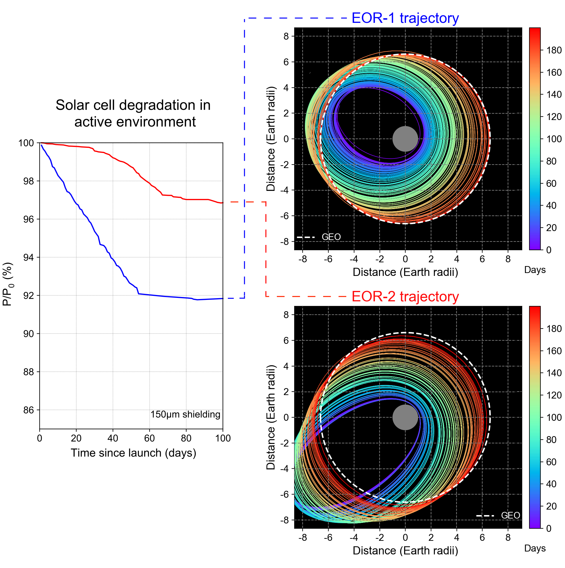
Figure caption: The left panel shows the remaining power, P/P0, as a function of time for two satellites. The right panels show trajectories of the two satellites over the first 200 mission days.
SuperDARN Observations During Geomagnetic Storms, Geomagnetically Active Times, and Enhanced Solar Wind Driving
by Maria-Theresia Walach (Lancaster University)
At Earth, solar wind coupling drives large scale convection of field lines: antisunward flow of open field lines at high latitudes and the return flow of closed field lines at lower latitudes. This convection can be observed through measurements of the ionosphere, for example using measurements from SuperDARN, an international network of ground based radars, purposely built to study ionospheric convection. We use 7 years of Super Dual Auroral Radar (SuperDARN) data to study ionospheric convection during geomagnetic storms, geomagnetically active times and solar wind driven times. Using the most recent years of SuperDARN data allows us to study ionospheric convection at the mid-latitudes with a field-of-view spanning from the pole to 40 degrees of magnetic latitude.
In this study, we address a number of questions; for example, do we make similar SuperDARN observations during similar solar wind driving during nonstorm time as during storm time? Do SuperDARN observations change throughout the different phases of a storm? Where do we see the fastest flows with SuperDARN, and is it linked to the extent of latitudinal coverage from the radars? Does the latitudinal range of the convection, given, for example, by the return flow region, stay constant throughout a storm? We find that initial and recovery phases of geomagnetic storms show similar convection as enhanced solar wind driving when no geomagnetic storm occurs.
One of the key findings showing the change of regime between the initial, main, and recovery phase of the storm is shown in the figure: it shows the varying relationship between the flow reversal boundary (here FRB but otherwise known as the open-closed field line boundary or polar cap boundary) and the Heppner-Maynard boundary (here HMB, which corresponds to the lower latitude boundary where the ionospheric convection electric field approaches 0 kV). The blue line shows the line of best fit and the data distribution along it, indicates that the boundaries must expand and contract together, however, this happens at different rates during the different storm phases, producing an inflated return flow region during the main phase of the storm.
For more information, please see the paper below:
, & ( 2019). SuperDARN observations during geomagnetic storms, geomagnetically active times, and enhanced solar wind driving. Journal of Geophysical Research: Space Physics, 124. https://doi.org/10.1029/2019JA026816
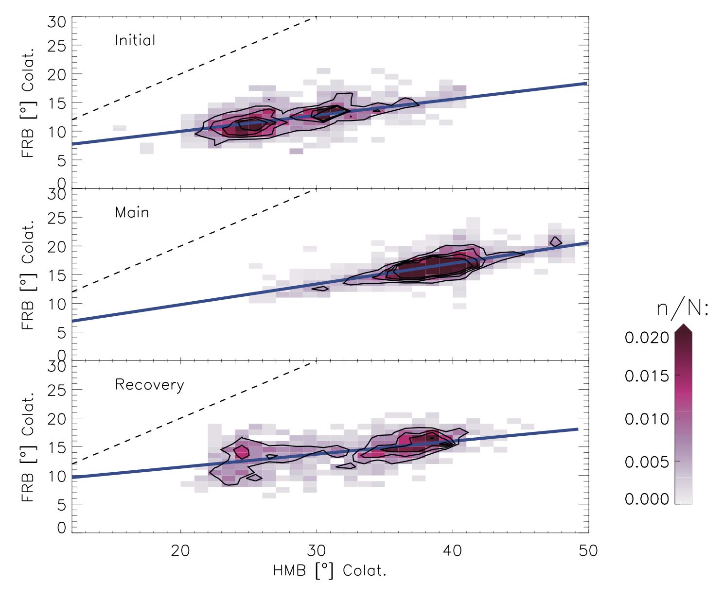
Figure: Colatitude location of the flow reversal boundary (FRB) against the Heppner‐Maynard boundary (HMB) during the three phases of geomagnetic storms (only using maps where n ≥ 200). The dashed black lines show the line of unity and the black contours correspond to where the normalized data point density corresponds to 0.005, 0.01, 0.015, and 0.02.
Exploring Key Characteristics in Saturn’s Infrared Auroral Emissions Using VLT-CRIRES: H3+ Intensities, Ion Line-of-Sight Velocities, and Rotational Temperatures
by Nahid Chowdhury (University of Leicester)
Saturn’s aurorae are generated by interactions between high-energy charged particles and neutral atoms in the upper atmosphere. Infrared observations of auroral emissions make use of H3+ – a dominant hydrogen ion in Saturn’s ionosphere – that acts as a tracer of energy injected into the ionosphere.
We analysed observations taken in May 2013 of Saturn’s northern infrared auroral emissions with the Very Large Telescope in Chile using the CRIRES instrument. The use of adaptive optics, combined with the high spectral resolution of VLT-CRIRES (100,000), meant that this dataset offered an unprecedented spatially and spectrally resolved ground-based view of Saturn's infrared aurora. Using discrete H3+ emission lines, we derived dawn-to-dusk auroral emission intensity, ion line-of-sight velocity, and thermospheric temperature profiles, allowing us to probe the physical properties of Saturn’s polar atmosphere.
Our analysis showed an enhancement in the dawn-side auroral emission intensity, a common feature that is known to be linked with solar-wind compressions in the kronian magnetosphere, and the presence of a localised dark region in the aurora very close to the pole. The ion line-of-sight velocity profile revealed previously unknown smaller-scale structures in the ion flows. In particular, the ion flows near the centre of the pole (at position B in Figure 1) could be consistent with the behaviour of a relatively small ionospheric polar vortex whereby the ions are interrupting the general dawn-to-dusk trend in movement to instead adopt a very sharp shearing motion of ions first toward midnight and then almost immediately back toward noon. Our thermospheric temperature derivations also reveal a very subtle temperature gradient that increases from 350 K on the dawn-side of the pole to 389 K on the dusk-side.
This work has bought to light complex features in the behaviour of H3+ ions in Saturn’s upper atmosphere for the first time and highlights the need for additional analyses of two-dimensional scanned maps of Saturn’s auroral regions with a view to addressing some of the major outstanding questions surrounding Saturn’s thermosphere-ionosphere-magnetosphere interaction.
For more information, please see the paper below:
, , , & ( 2019). Exploring key characteristics in Saturn's infrared auroral emissions using VLT‐CRIRES: H3+intensities, ion line‐of‐sight velocities, and rotational temperatures. Geophysical Research Letters, 46. https://doi.org/10.1029/2019GL083250.
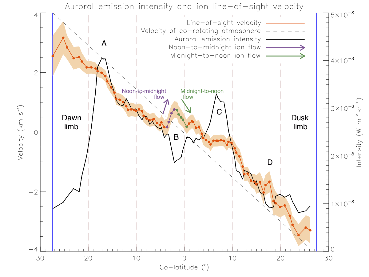
Figure 1: The ion line-of-sight velocity and auroral emission intensity profiles are plotted as a function of co-latitude on the planet. Evidence for ion flows possibly consistent with the behaviour of an intriguing ionospheric polar vortex is adjacent to the area marked by the letter B, between approximately 0⁰ and 5⁰ co-latitude on the dawn-side of Saturn’s northern pole.
Directed network of substorms using SuperMAG ground-based magnetometer data
by Lauren Orr (University of Warwick)
Space weather can cause large-scale currents in the ionosphere which generate disturbances of magnetic fields on the ground. These are observed by >100 magnetometer stations on the ground. Network analysis can extract the important information from these many observations and present it as a few key parameters that indicate how severe the ground impact will be. We quantify the spatio-temporal evolution of the substorm ionospheric current system utilizing the SuperMAG 100+ magnetometers, constructing dynamical directed networks from this data for the first time.
Networks are a common analysis tool in societal data, where people are linked based on various social relationships. Other examples of networks include the world wide web, where websites are connected via hyperlinks, or maps where places are linked via roads. We have constructed networks from the magnetometer observations of substorms, where magnetometers are linked if there is significant correlation between the observations. If the canonical cross-correlation (CCC) between vector magnetic field perturbations observed at two magnetometer stations exceeds a threshold, they form a network connection. The time lag at which CCC is maximal, |τC|, determines the direction of propagation or expansion of the structure captured by the network connection. If spatial correlation reflects ionospheric current patterns, network properties can test different models for the evolving substorm current system.
In this study, we select 86 isolated substorms based on nightside ground station coverage. The results are shown for both a single event and for all substorms in the figure. We find, and obtain the timings for, a consistent picture in which the classic substorm current wedge (SCW) forms, quantifying both formation and expansion. A current system is seen pre-midnight following the SCW westward expansion. Later, there is a weaker signal of eastward expansion. Finally, there is evidence of substorm-enhanced magnetospheric convection. These results demonstrate the capabilities of network analysis to understand magnetospheric dynamics and provide new insight into how the SCW develops and evolves during substorms.
For more information please see the paper below:
Orr, L., Chapman, S. C., and Gjerloev, J. W.. ( 2019), Directed network of substorms using SuperMAG ground‐based magnetometer data. Geophys. Res. Lett., 46. https://doi.org/10.1029/2019GL082824

Figure: The normalized number of connections, α(t',τC), is binned by the lag of maximal canonical cross-correlation, |τC|. Each panel stacks, one above the other, α(t',τC) versus normalized time, t’, for |τC|≤15. The regions are indicated on the polar plot and the regions were determined using Polar VIS images of the auroral bulge at the time of maximum expansion. Region B (around onset) exhibits a rapid increase in correlation following substorm onset.